


目录
说明:为了复习高数,该文章是学习课程 《高等数学》同济版 全程教学视频(宋浩老师)而记录的笔记,笔记、MATLAB代码来源于本人。若有侵权,请联系本人删除。笔记难免可能出现错误或笔误,若读者发现笔记有错误,欢迎在评论里批评指正。参考书籍: 高等数学下册(同济_第7版)。
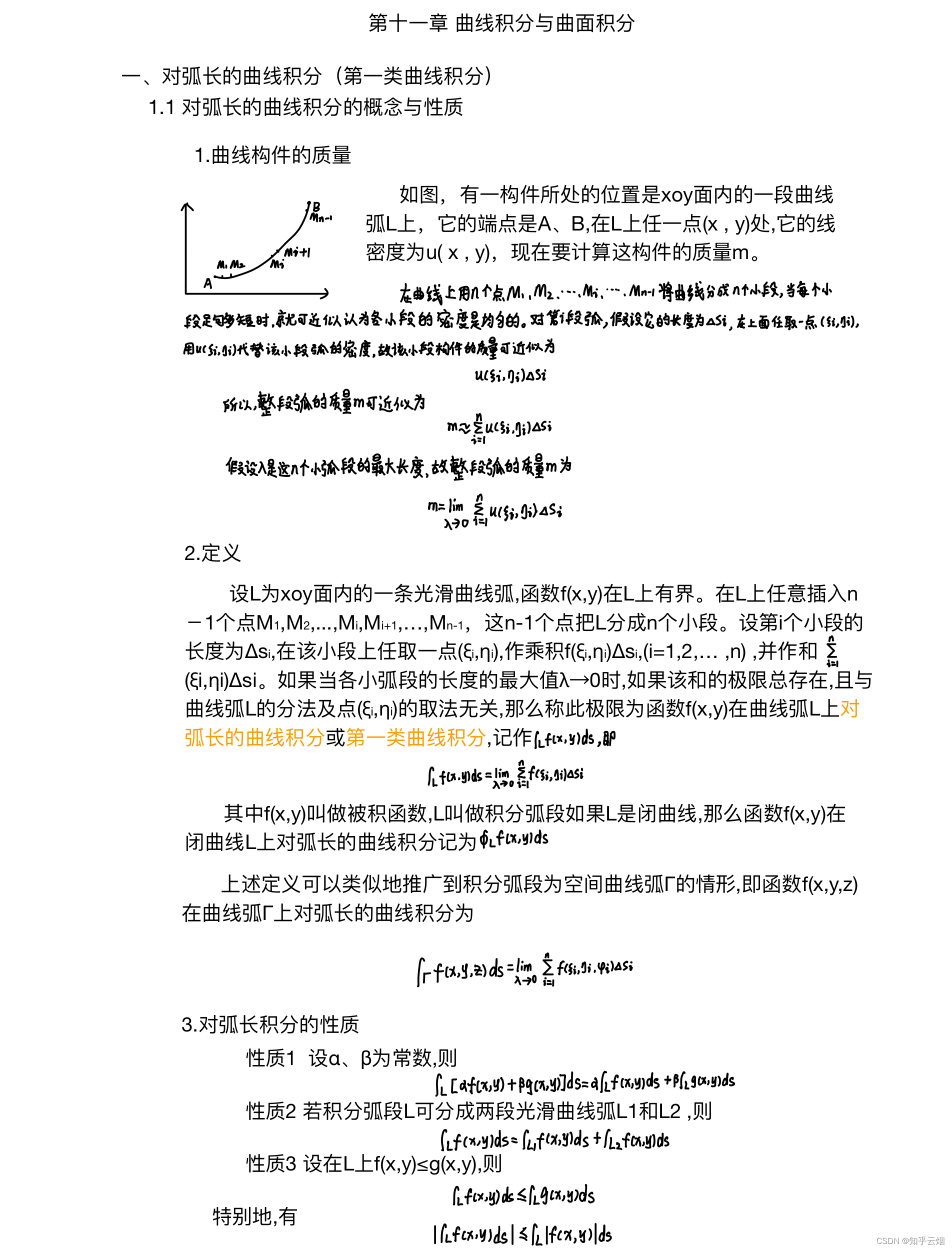
一、对弧长的曲线积分
1.1 对弧长曲线积分的概念与性质(引例(求曲线构件的质量)、定义、性质)
1.2 对弧长的曲线积分的计算法(参数方程下的曲线积分)
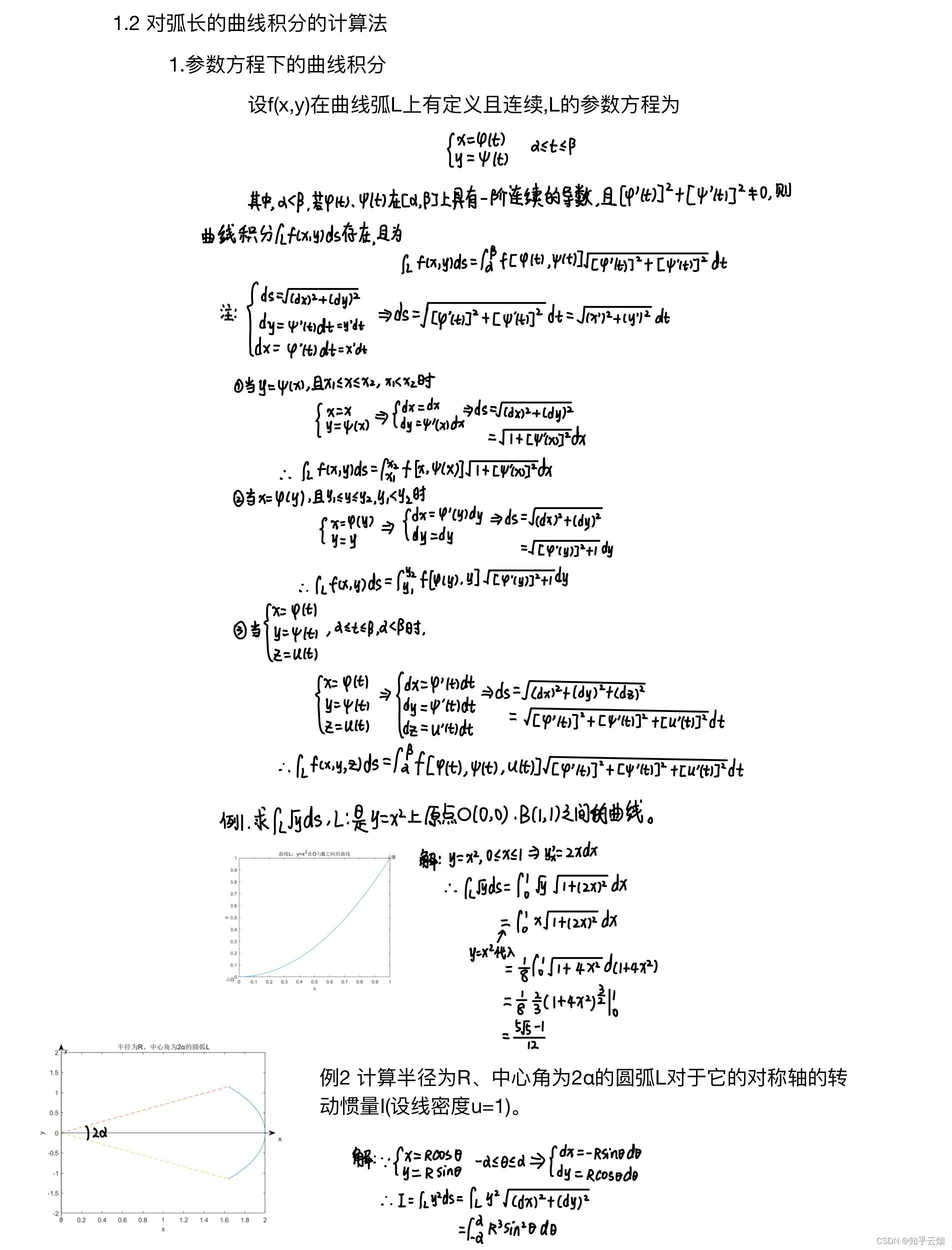
例1的代码:
clc;
clear ;
close all;
x = linspace(0,1,20);
y = x.^2;
figure;
plot(x,y)
xlabel('x');
ylabel('y');
title('曲线L:y=x^2在O与B之间的曲线');
text(0-0.06,0-0.02,'点O','HorizontalAlignment','center')
text(1+0.01,1+0.01,'点B','HorizontalAlignment','center')
例2的代码:
clc;
clear ;
close all;
% 1.基本图形
R = 2;
alpha_0 = -35:0.2:35;
alpha = alpha_0/180*pi;
x = R*cos(alpha);
y = R*sin(alpha);
figure;
plot(x,y);
hold on;
x1 = linspace(0,R*cos(alpha(end)),50);
y1 = x1*tan(alpha(end));
y2 = -x1*tan(alpha(end));
plot(x1,y1,'--');plot(x1,y2,'--');
xlabel('x');
ylabel('y');
title('半径为R、中心角为2α的圆弧L');

% 2.x轴与y轴
% 2.1 x轴
% ------------x 轴参数(注意理解)------------------
axis([0 2 -2 2]);
p1=[0 0];p2=[2.1 0];%从点(0,0)到(2.1,0),根据需要进行调整
%坐标转换,将点p1、p2实际axes坐标转成figure坐标
% 获取 Axes 位置
posAxes = get(gca, 'Position');
posX = posAxes(1);
posY = posAxes(2);
width = posAxes(3);
height = posAxes(4);
% 获取 Axes 范围
limX = get(gca, 'Xlim');
limY = get(gca, 'Ylim');
minX = limX(1);
maxX = limX(2);
minY = limY(1);
maxY = limY(2);
% 转换坐标
xNew1 = posX + (p1(1) - minX) / (maxX - minX) * width;
xNew2 = posX + (p2(1) - minX) / (maxX - minX) * width;
yNew1 = posY + (p1(2) - minY) / (maxY - minY) * height;
yNew2 = posY + (p2(2) - minY) / (maxY - minY) * height;
% -------------画x轴----------------------------
annotation(gcf, 'arrow', [xNew1 xNew2], [yNew1 yNew2]);
annotation(gcf, 'textbox',[xNew2 yNew2 0 0], 'String', 'x', 'EdgeColor', 'none');
% 2.2 y轴
p1=[0 -2.2];p2=[0 2.2];%从点(0,-2.2)到(0,2.2),根据需要进行调整
%坐标转换,将点p1、p2实际axes坐标转成figure坐标
% 获取 Axes 位置
posAxes = get(gca, 'Position');
posX = posAxes(1);
posY = posAxes(2);
width = posAxes(3);
height = posAxes(4);
% 获取 Axes 范围
limX = get(gca, 'Xlim');
limY = get(gca, 'Ylim');
minX = limX(1);
maxX = limX(2);
minY = limY(1);
maxY = limY(2);
% 转换坐标
xNew1 = posX + (p1(1) - minX) / (maxX - minX) * width;
xNew2 = posX + (p2(1) - minX) / (maxX - minX) * width;
yNew1 = posY + (p1(2) - minY) / (maxY - minY) * height;
yNew2 = posY + (p2(2) - minY) / (maxY - minY) * height;
% -------------画y轴----------------------------
annotation(gcf, 'arrow', [xNew1 xNew2], [yNew1 yNew2]);
annotation(gcf, 'textbox',[xNew2 yNew2 0 0], 'String', 'y', 'EdgeColor', 'none');

hold off;
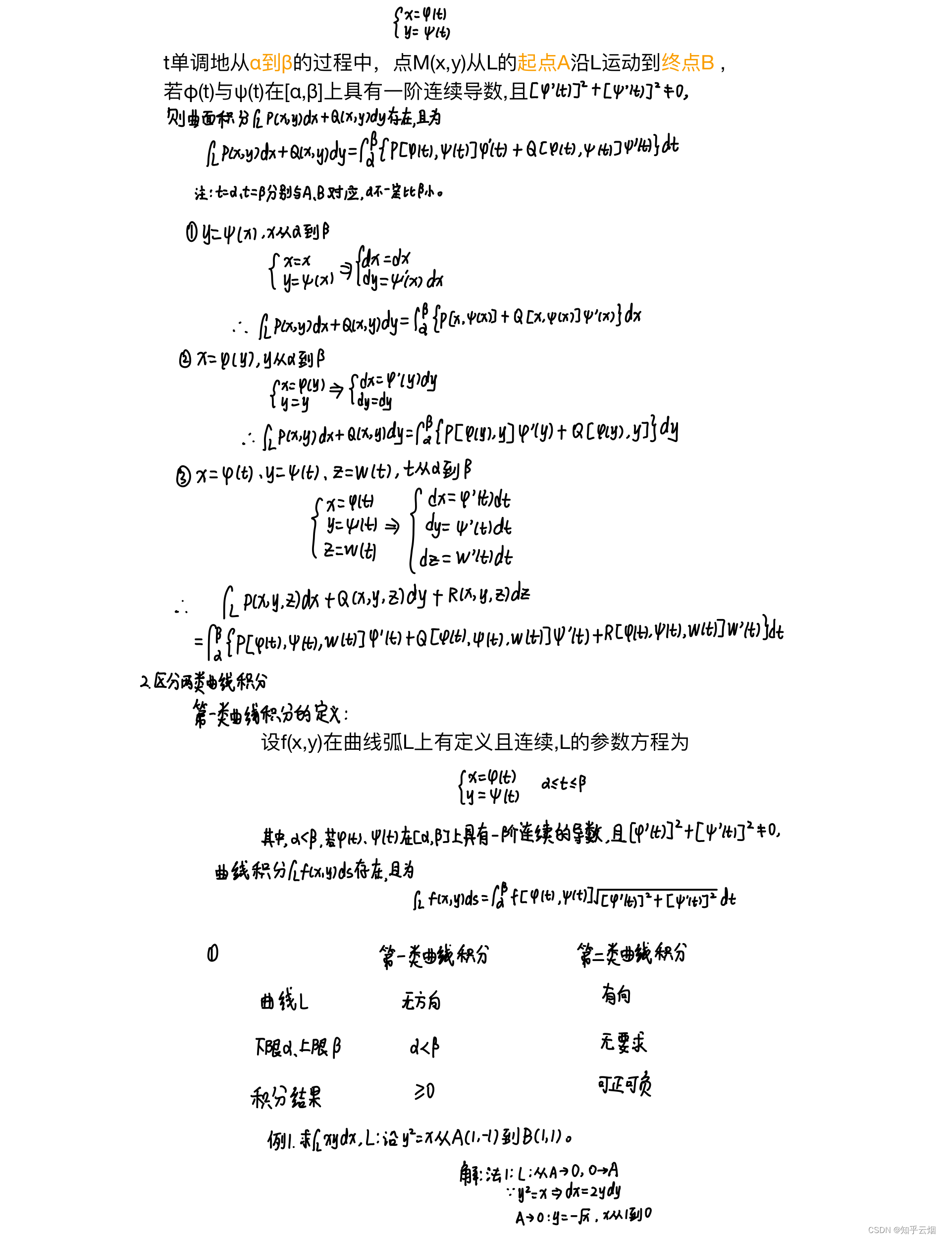
二、对坐标的曲线积分
2.1 对坐标的曲线积分的概念与性质(引例(变力沿曲线所作的功)、定义、性质)
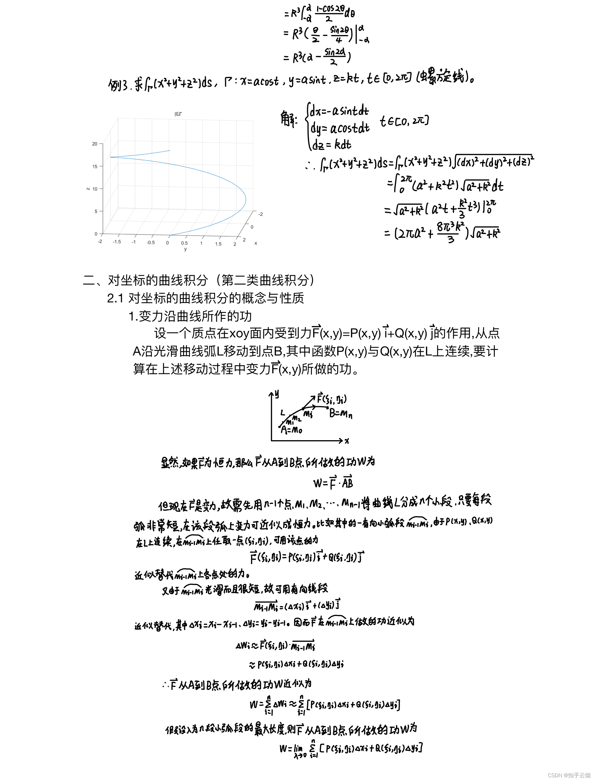
例3的代码:
clc;
clear ;
close all;
a = 2;k = 3;
t = linspace(0,2*pi,100);
x = a*cos(t);
y = a*sin(t);
z = k*t;
figure;
plot3(x,y,z);
hold on;
xlabel('x');
ylabel('y');
zlabel('z');
title('弧Γ');
grid on;
hold off;
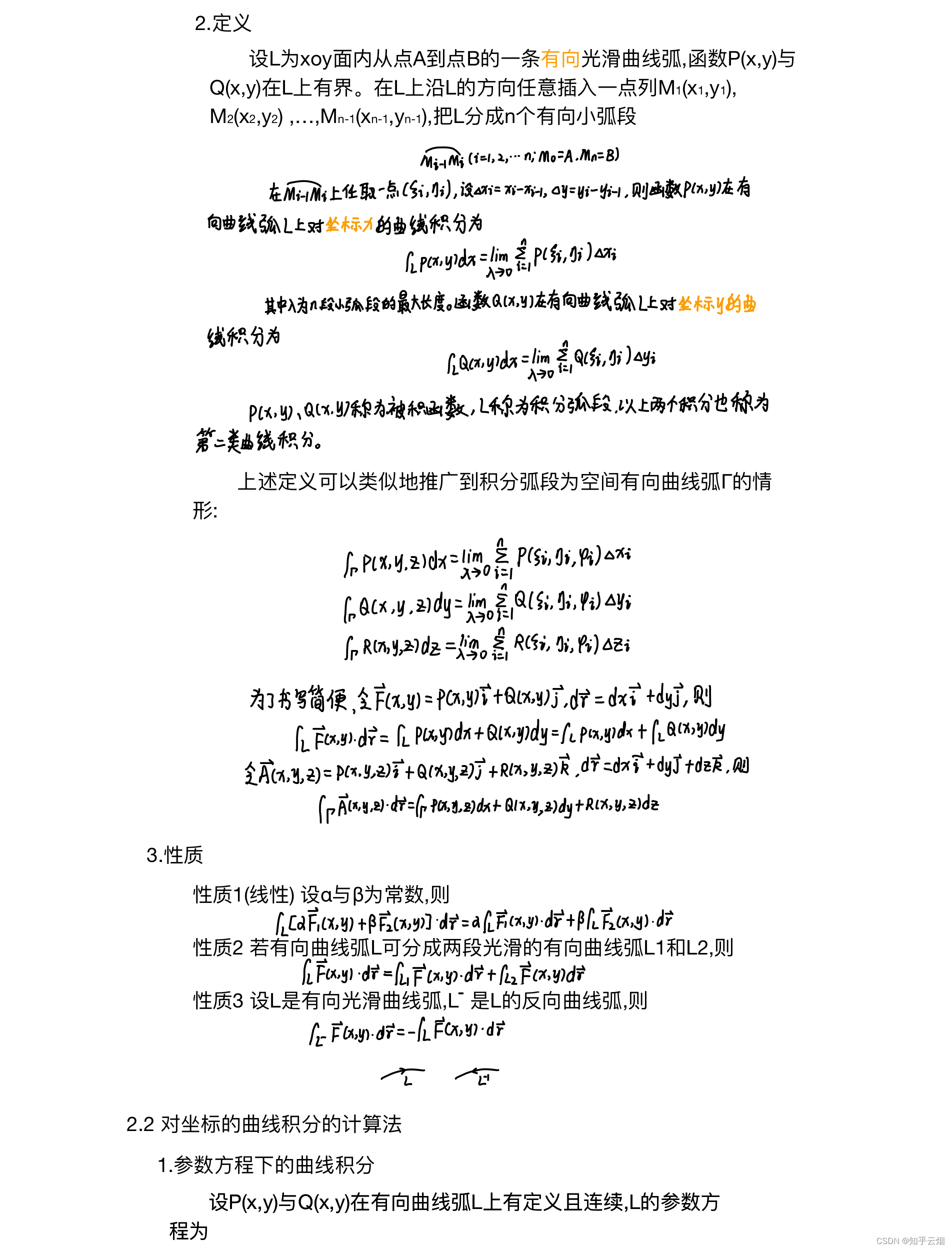
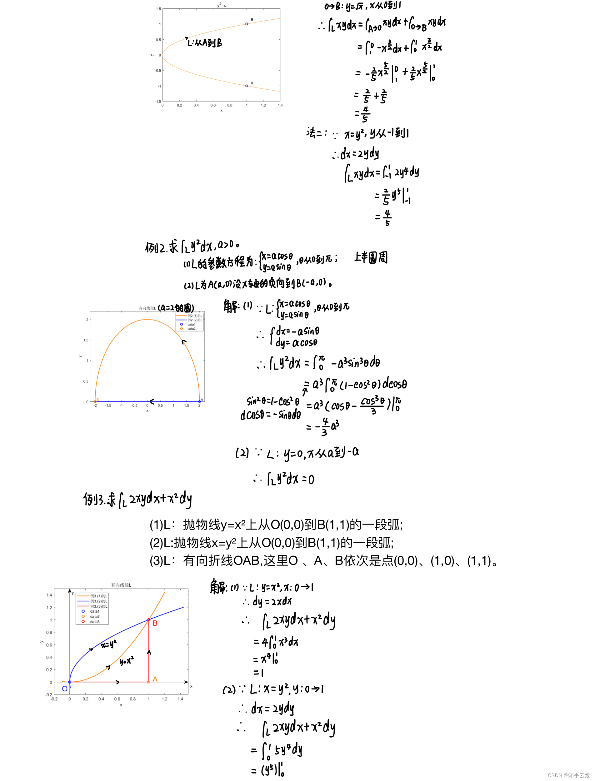
2.2 对坐标的曲线积分的计算法(参数方程下的曲线积分、两类曲线积分的区分)
例1的代码:
clc;
clear ;
close all;
% 1.绘制 y^2=x 曲线
x = 0:0.01:1.4;
y1 = sqrt(x);
y2 = -sqrt(x);
figure;
plot(x,y1,'color',[1 0.5 0]);% 橙色线
hold on; % 保留绘图
plot(x,y2,'color',[1 0.5 0]);
xlabel('x');
ylabel('y');
title('y^2=x');
% 2.在点 A 和点 B 上进行标注
O = [1, -1];
A = [1, 1];
plot(O(1), O(2), 'bo','LineWidth',1.5); % 在点A处画出一个蓝色圆点
text(O(1)+0.05, O(2)+0.1, 'A'); % 在点A处写上文字"A"
plot(A(1), A(2), 'bo','LineWidth',1.5); % 在点 B 处画出一个蓝色圆点
text(A(1)+0.05, A(2)+0.15, 'B'); % 在点B处写上文字"B"
hold off;
例2的代码:
clc;
clear ;
close all;
% 1.绘制(1)的L
theta = linspace(0,pi,50);
a = 2;
x1 = 2*cos(theta);
y1 = 2*sin(theta);
figure;
plot(x1,y1,'color',[1 0.5 0],'LineWidth',1.5);% 橙色线
hold on; % 保留绘图
xlabel('x');
ylabel('y');
% 2.绘制(2)的L
x2 = x1;
y2 = zeros(size(x2));
plot(x2,y2,'color','b','LineWidth',1.5);% 蓝色线
legend('例2.(1)的L','例2.(2)的L');
% 3.在点 A 和点 B 上进行标注
O = [a, 0];
A = [-a, 0];
plot(O(1), O(2), 'bo','LineWidth',1.5); % 在点A处画出一个蓝色圆点
text(O(1)+0.05, O(2)+0.05, 'A','Color','b'); % 在点A处写上文字"A"
plot(A(1), A(2), 'o','Color',[1 0.5 0],'LineWidth',1.5); % 在点 B 处画出一个橙色圆点
text(A(1)+0.05, A(2)+0.05, 'B','Color',[1 0.5 0]); % 在点B处写上文字"B"
axis([-2.2 2.2 0 2.2]);
title('有向线段L');
hold off;
例3的代码:
clc;
clear ;
close all;
% 1.绘制(1)的L: 抛物线y=x^2上从O(0,0)到B(1,1)的一段弧
x1 = -0.1:0.02:1.2;
y1 = x1.^2;
figure;
plot(x1,y1,'color',[1 0.5 0],'LineWidth',1.5);% 橙色线
hold on; % 保留绘图
xlabel('x');
ylabel('y');
% 3.绘制(2)的L: 抛物线x=y^2上从O(0,0)到B(1,1)的一段弧
y2 = -0.1:0.02:1.2;
x2 = y2.^2;
plot(x2,y2,'color','b','LineWidth',1.5);% 蓝线
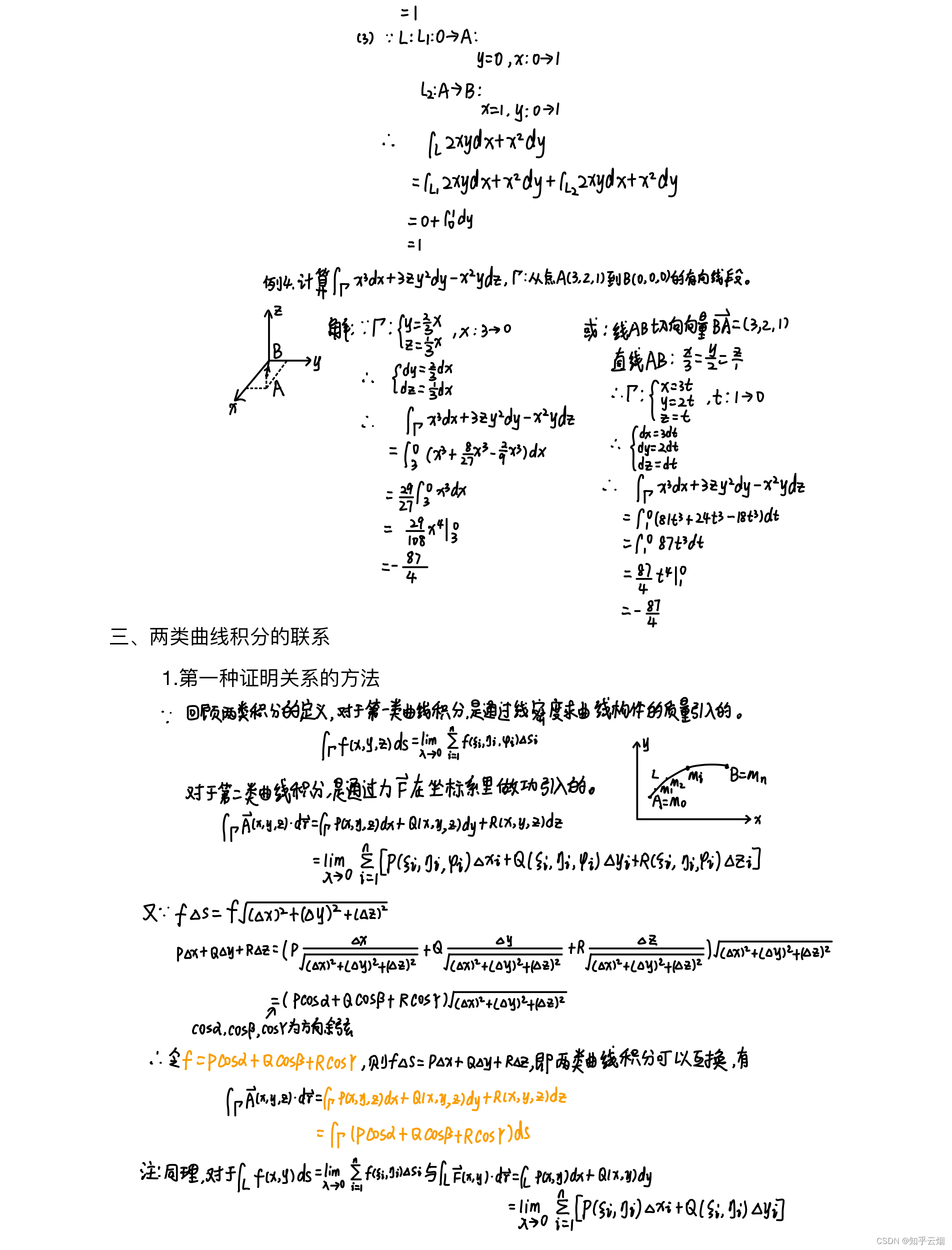
% 3.绘制(3)的L: 有向折线OAB,这里О 、A、B依次是点(0,0)、(1,0)、(1,1)
x3 = 0:0.01:1;
y3 = 0*ones(size(x3));
x4 = linspace(1,1,50);
y4 = linspace(0,1,length(x4));
plot(x3,y3,'color','r','LineWidth',1.5);
plot(x4,y4,'color','r','LineWidth',1.5);
legend('例3.(1)的L','例3.(2)的L','例3.(3)的L');
% 4.在点O、A、B上进行标注
O = [0,0];
A = [1,0];
B = [1,1];
plot(O(1), O(2), 'bo','LineWidth',1.5); % 在点O处画出一个蓝色圆点
text(O(1)-0.1, O(2)-0.1, 'O','Color','b','FontSize',18); % 在点O处写上文字"O"
plot(A(1), A(2), 'o','Color',[1 0.5 0],'LineWidth',1.5); % 在点 A 处画出一个橙色圆点
text(A(1)+0.05, A(2)+0.05, 'A','Color',[1 0.5 0],'FontSize',18); % 在点B处写上文字"A"
plot(B(1), B(2), 'o','Color','r','LineWidth',1.5); % 在点 B 处画出一个橙色圆点
text(B(1)+0.05, B(2)-0.05, 'B','Color','r','FontSize',18); % 在点B处写上文字"B"
title('有向线段L');
axis([-0.2 1.5 -0.2 1.5]);
% 5.x轴与y轴
% 5.1 x轴
% ------------x 轴参数(注意理解)------------------
p1=[-0.2 0];p2=[1.5 0];%从点p1到p2,根据需要进行调整
%坐标转换,将点p1、p2实际axes坐标转成figure坐标
% 获取 Axes 位置
posAxes = get(gca, 'Position');
posX = posAxes(1);
posY = posAxes(2);
width = posAxes(3);
height = posAxes(4);
% 获取 Axes 范围
limX = get(gca, 'Xlim');
limY = get(gca, 'Ylim');
minX = limX(1);
maxX = limX(2);
minY = limY(1);
maxY = limY(2);
% 转换坐标
xNew1 = posX + (p1(1) - minX) / (maxX - minX) * width;
xNew2 = posX + (p2(1) - minX) / (maxX - minX) * width;
yNew1 = posY + (p1(2) - minY) / (maxY - minY) * height;
yNew2 = posY + (p2(2) - minY) / (maxY - minY) * height;
% -------------画x轴----------------------------
annotation(gcf, 'arrow', [xNew1 xNew2], [yNew1 yNew2]);
annotation(gcf, 'textbox',[xNew2 yNew2 0 0], 'String', 'x', 'EdgeColor', 'none');
% 5.2 y轴
p1=[0 -0.2];p2=[0 1.5];%从点p1到p2,根据需要进行调整
%坐标转换,将点p1、p2实际axes坐标转成figure坐标
% 获取 Axes 位置
posAxes = get(gca, 'Position');
posX = posAxes(1);
posY = posAxes(2);
width = posAxes(3);
height = posAxes(4);
% 获取 Axes 范围
limX = get(gca, 'Xlim');
limY = get(gca, 'Ylim');
minX = limX(1);
maxX = limX(2);
minY = limY(1);
maxY = limY(2);
% 转换坐标
xNew1 = posX + (p1(1) - minX) / (maxX - minX) * width;
xNew2 = posX + (p2(1) - minX) / (maxX - minX) * width;
yNew1 = posY + (p1(2) - minY) / (maxY - minY) * height;
yNew2 = posY + (p2(2) - minY) / (maxY - minY) * height;
% -------------画y轴----------------------------
annotation(gcf, 'arrow', [xNew1 xNew2], [yNew1 yNew2]);
annotation(gcf, 'textbox',[xNew2 yNew2 0 0], 'String', 'y', 'EdgeColor', 'none');
hold off;
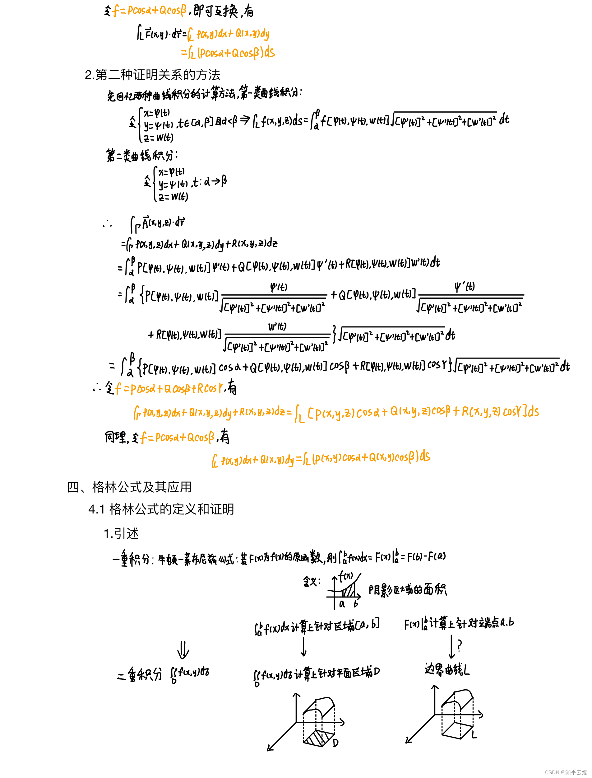
三、两类曲线积分的联系(两种证明联系的方法)
四、格林公式及其应用
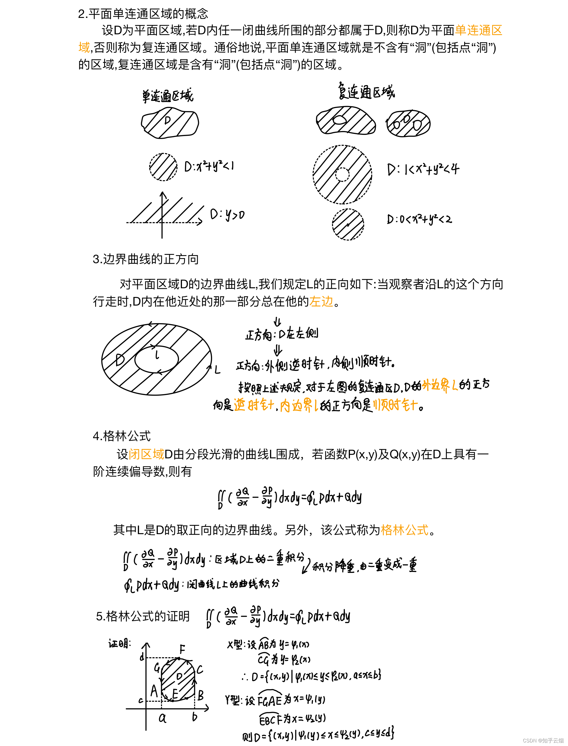
4.1 格林公式的定义和证明(引述、平面单连通区域的概念、边界曲线的正方向、格林公式的定义及证明)
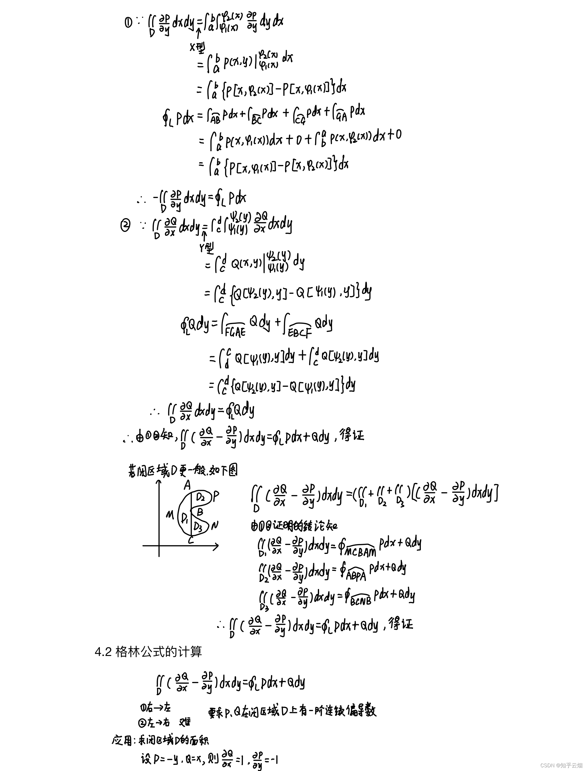
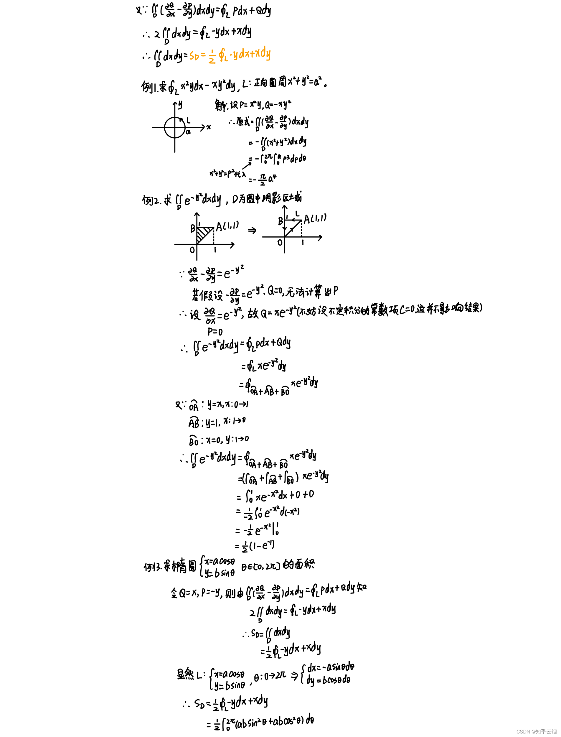
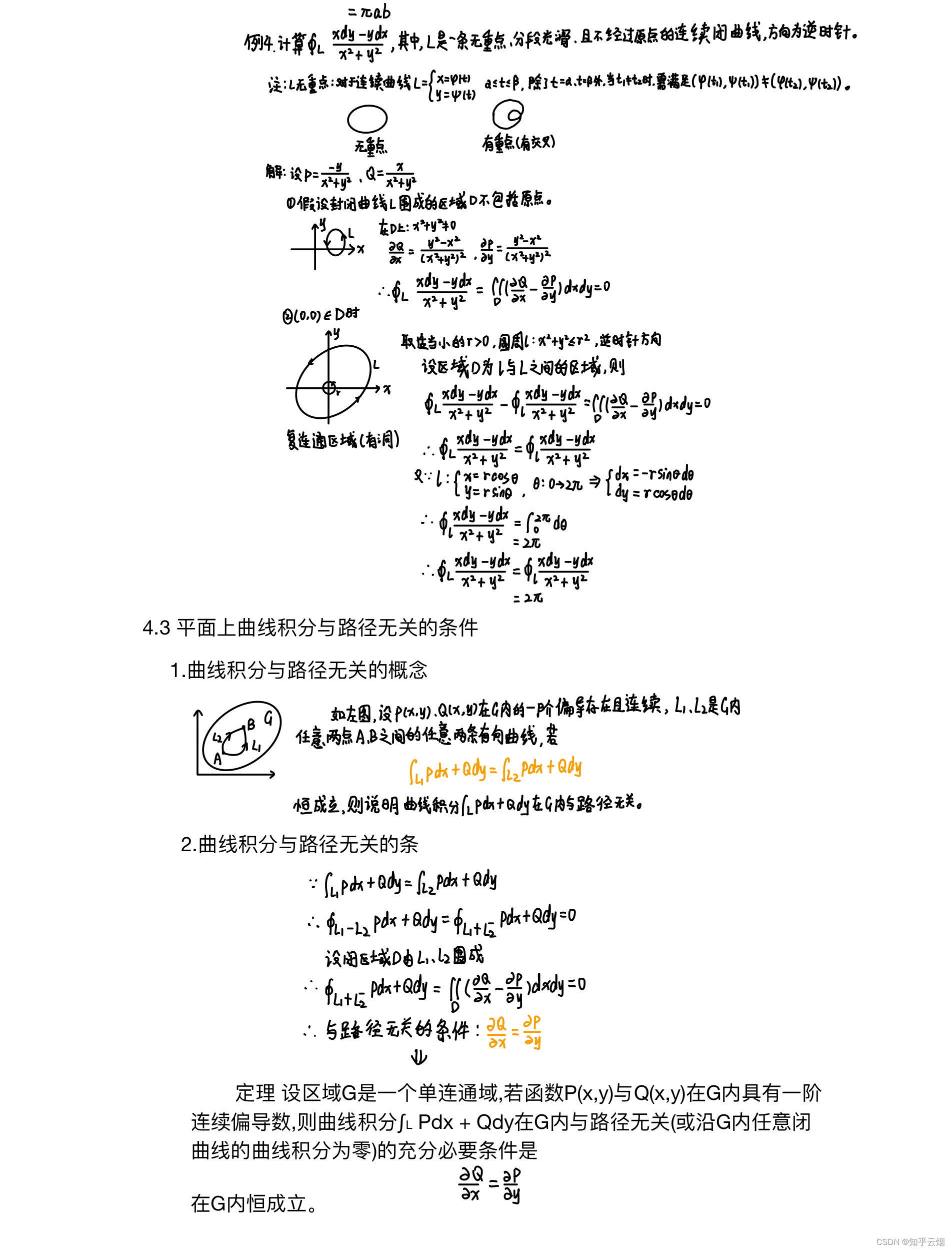
4.2 格林公式的计算
4.3 平面上曲线积分与路径无关的概念、条件
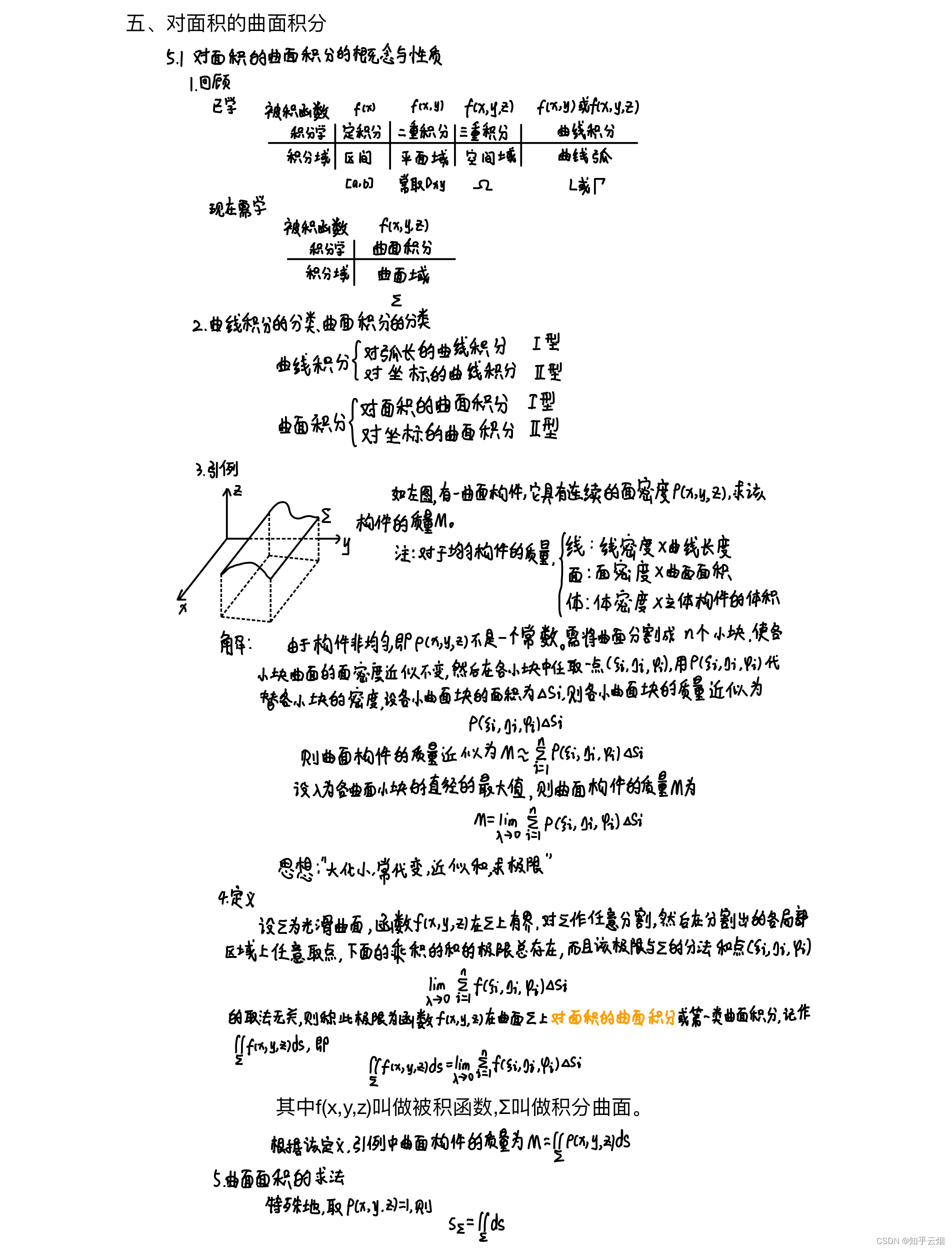
五、对面积的曲面积分
5.1 对面积的曲面积分的概念与性质(回顾、曲线积分的分类、曲面积分的分类、引例(求曲面构件的质量)、定义、曲面面积的求法、性质(积分的存在性、积分区域的可加性、线性、不等式关系))
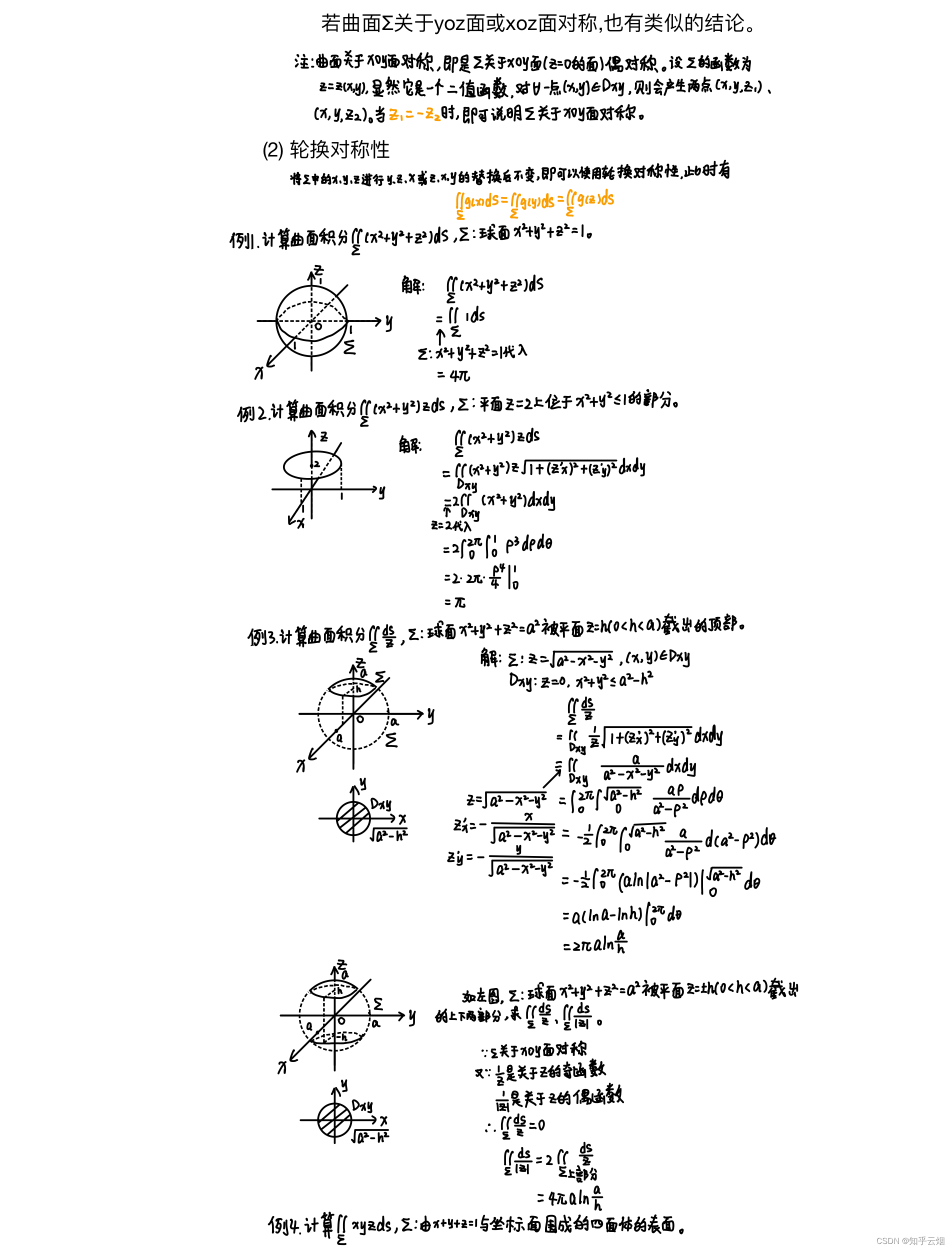
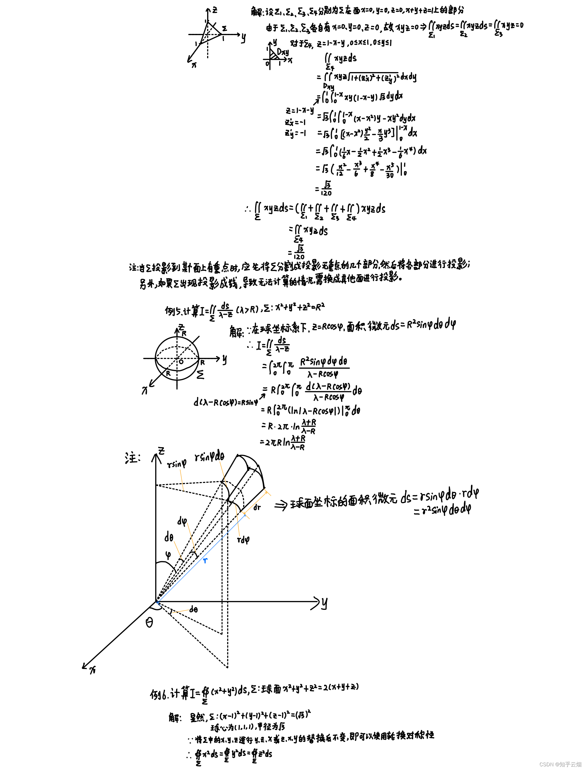
5.2 对面积的曲面积分的计算法(计算步骤(“一投二代三微变”)、投影面的一般选取规则、利用性质简化运算(奇偶性、轮换对称性、有的题可用质心公式进行简化))

六、对坐标的曲面积分
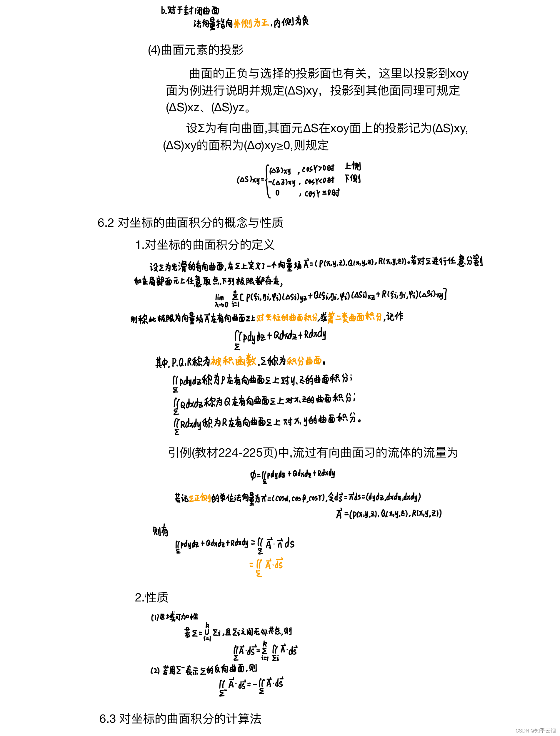
6.1 有向曲面的定义、分类、方向及曲面元素的投影
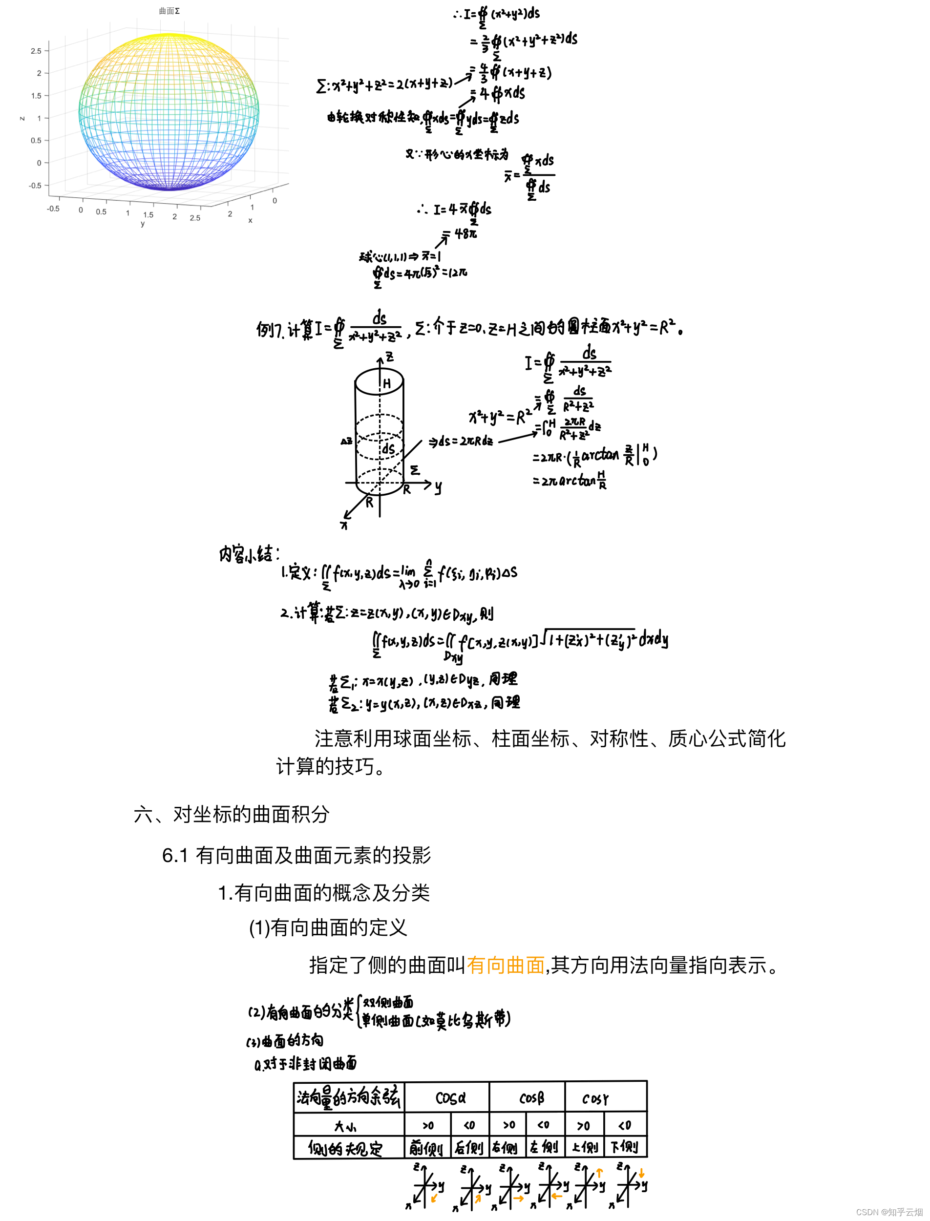
例6的代码:
clc;
clear ;
close all;
% 1.Σ的参数方程
n = 50;
theta = linspace(0,2*pi,n);
phi = linspace(0,pi,n/2);
[theta,phi] = meshgrid(theta,phi);
x = sqrt(3)*sin(phi).*cos(theta)+1;
y = sqrt(3)*sin(phi).*sin(theta)+1;
z = sqrt(3)*cos(phi)+1;
% 2.画图
figure;
mesh(x,y,z);
hold on;
xlabel('x');
ylabel('y');
zlabel('z');
title('曲面Σ');
grid on;
axis tight;
hidden off %打开透视
hold off;
6.2 对坐标的曲面积分的概念与性质(定义、性质)
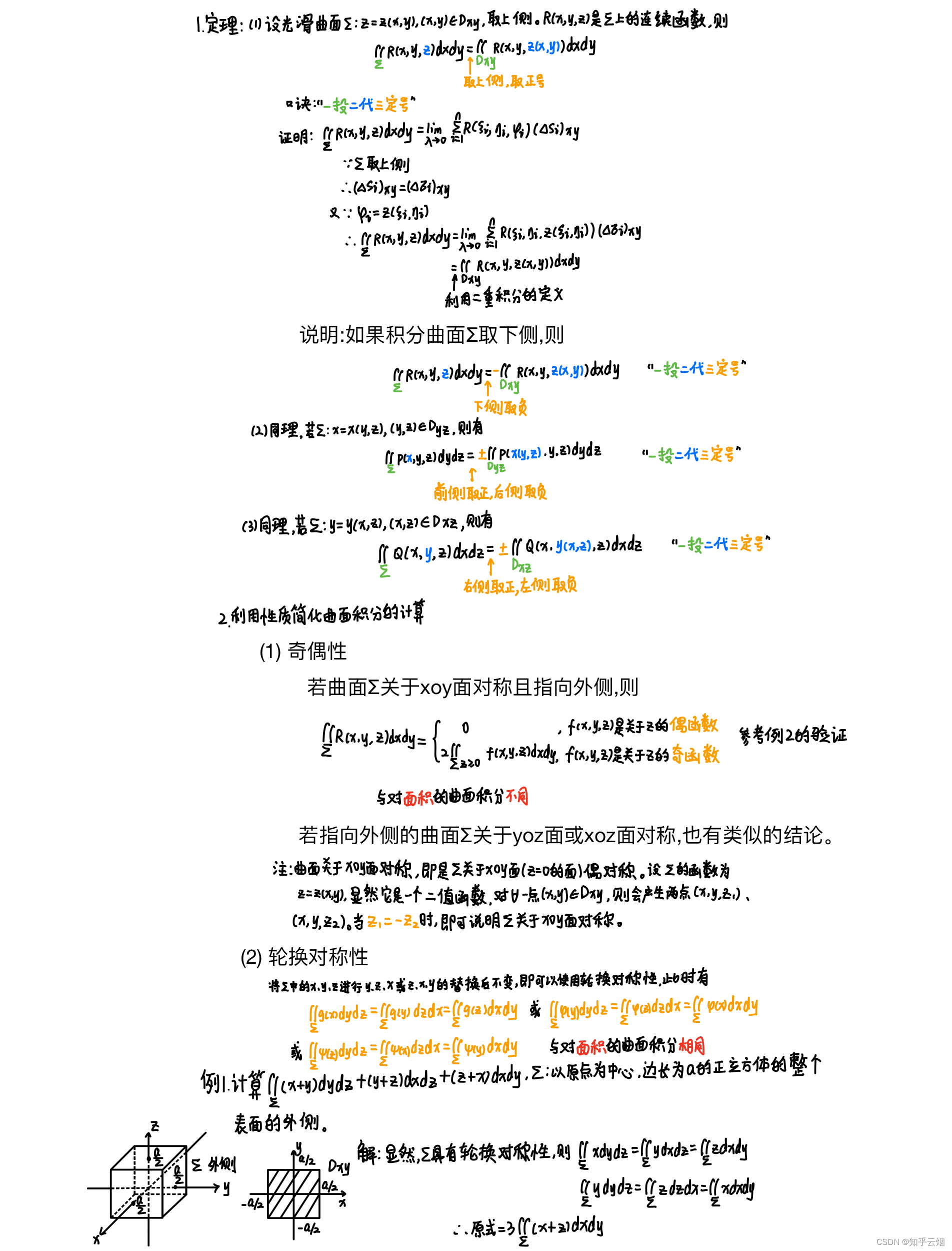
6.3 对坐标的曲面积分的计算法(步骤(“一投二代三定号”)、利用性质简化计算(奇偶性、轮换对称性))
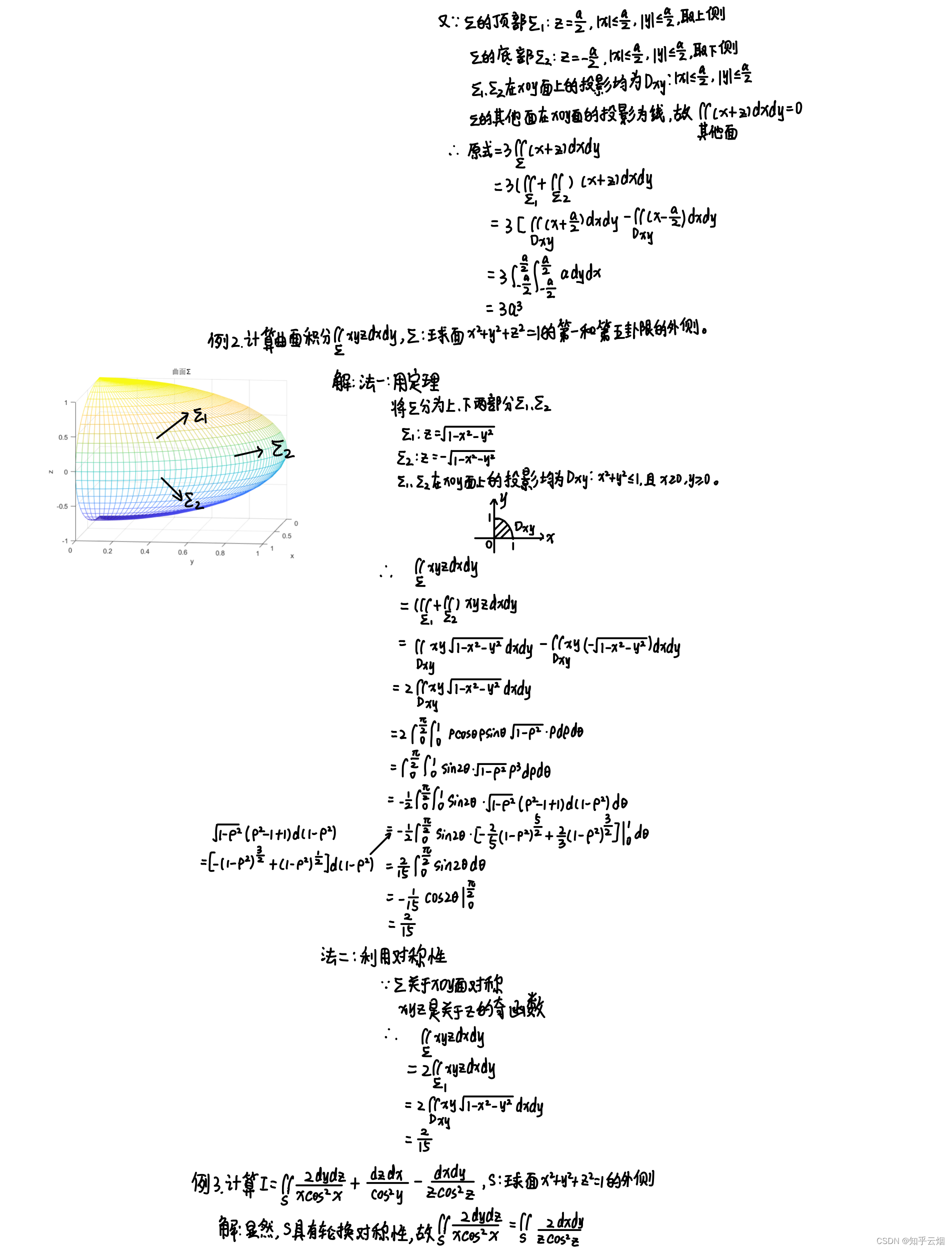
例2的代码:
clc;
clear ;
close all;
% 1.Σ的参数方程
n = 50;
theta = linspace(0,1/2*pi,n);
phi = linspace(0,pi,n/2);
[theta,phi] = meshgrid(theta,phi);
x = 1*sin(phi).*cos(theta);
y = 1*sin(phi).*sin(theta);
z = 1*cos(phi);
% 2.画图
figure;
mesh(x,y,z);
hold on;
xlabel('x');
ylabel('y');
zlabel('z');
title('曲面Σ');
grid on;
axis tight;
hidden off %打开透视
hold off;
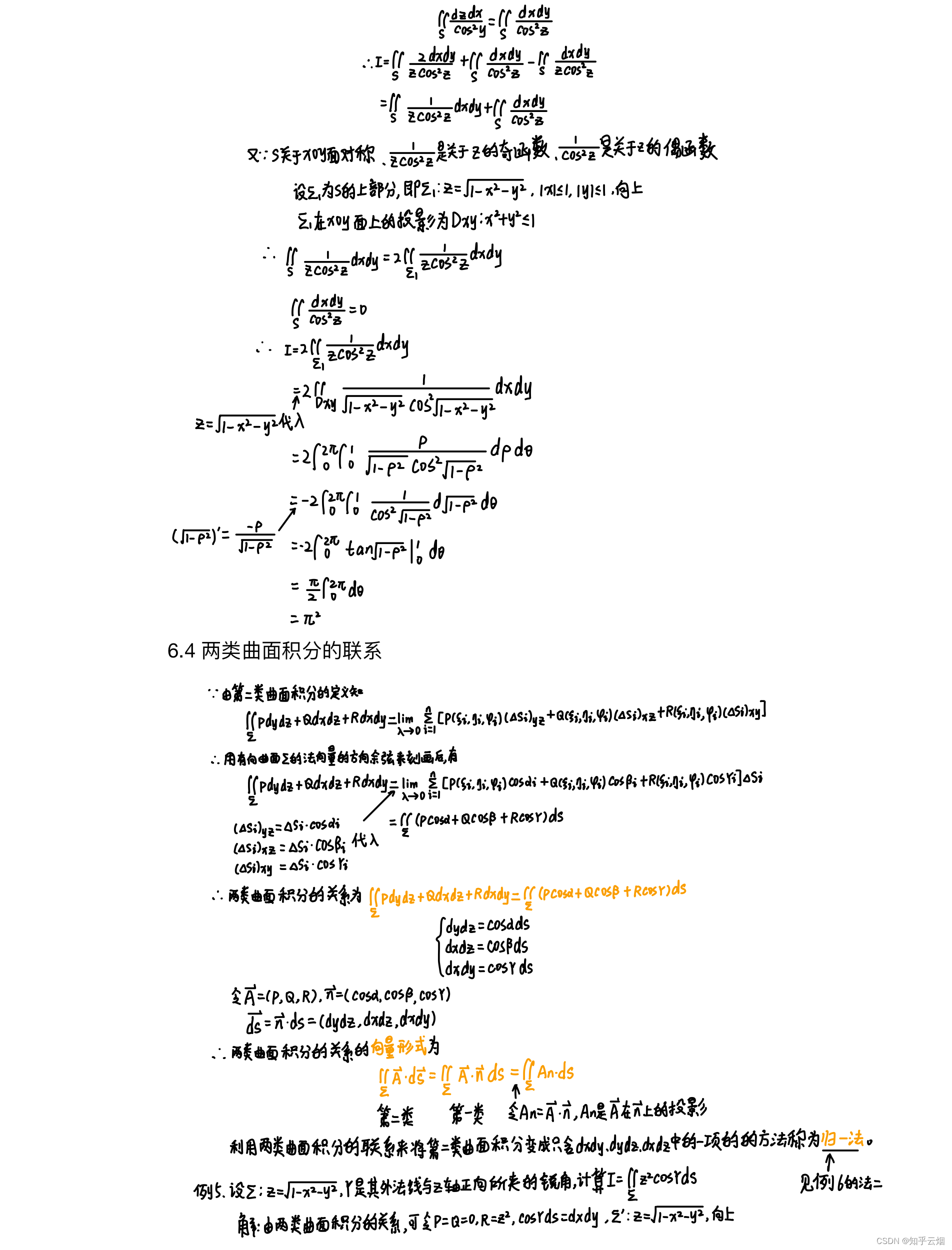
6.4 两类曲面积分的联系
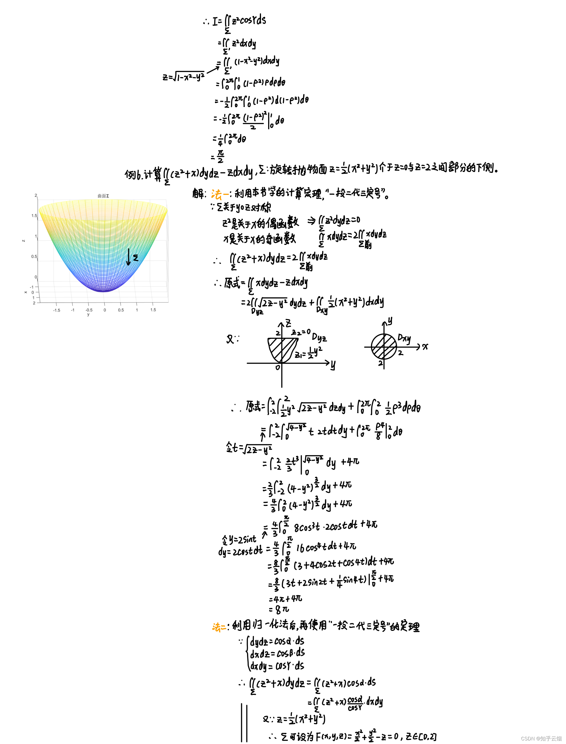
例6的代码:
clc;
clear ;
close all;
% 1.曲面Σ的参数方程
theta = linspace(0,2*pi,60);
z = linspace(0,2,80);
[theta,z]=meshgrid(theta,z);
x = sqrt(2*z).*cos(theta);
y = sqrt(2*z).*sin(theta);
% 2.画图
figure;
mesh(x,y,z);
hold on;
xlabel('x');
ylabel('y');
zlabel('z');
title('曲面Σ');
grid on;
axis tight;
hidden off %打开透视
hold off;
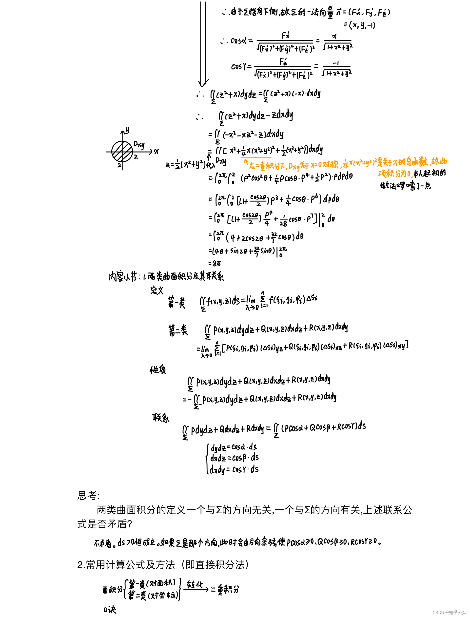
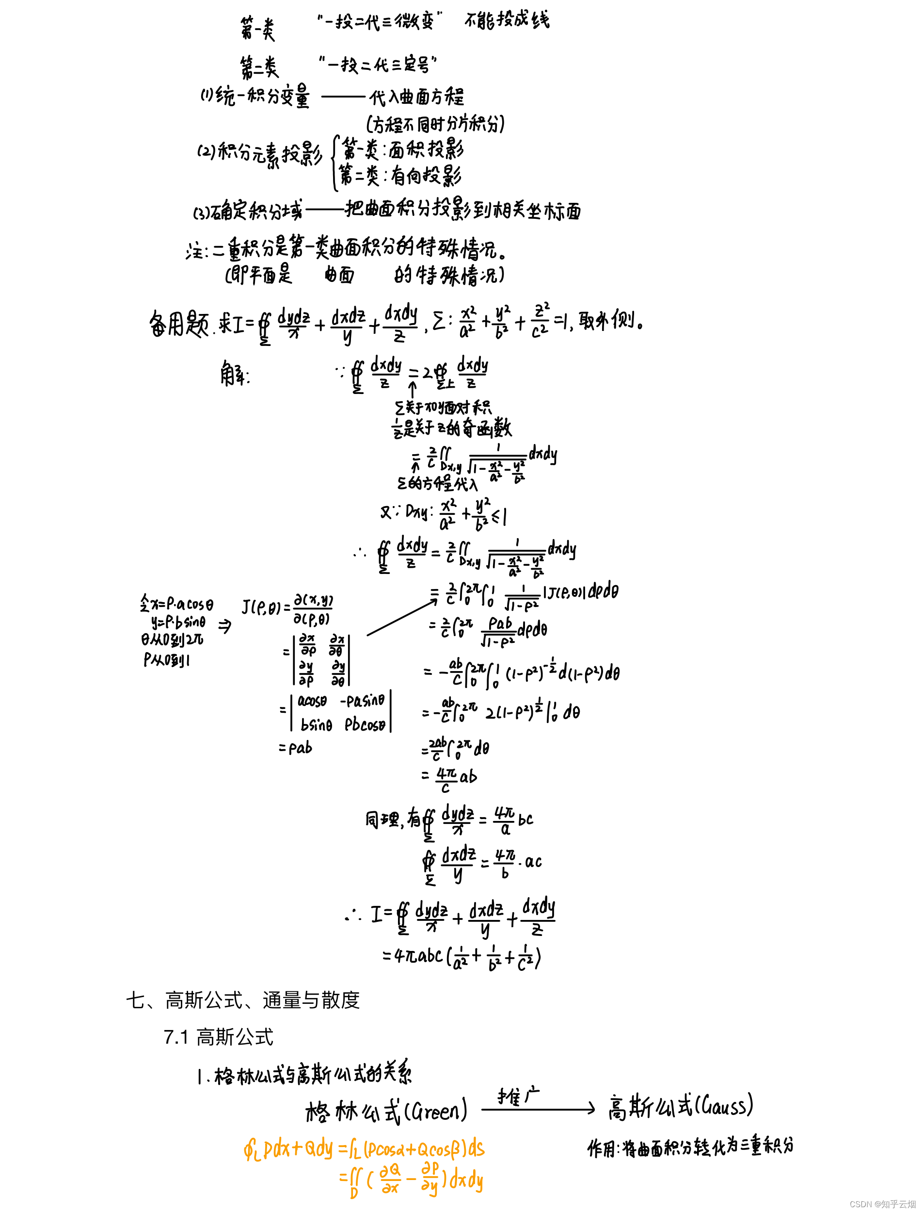
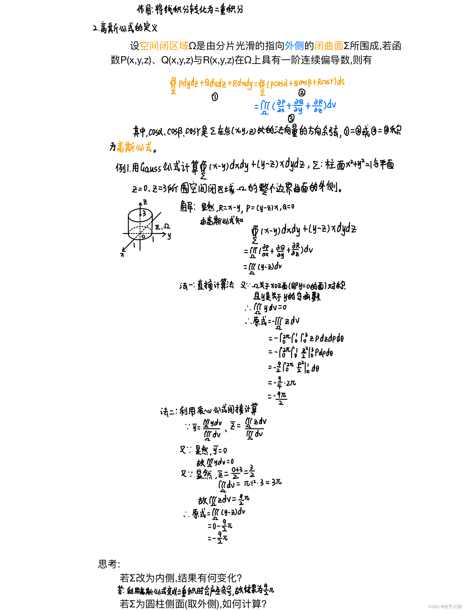
七、高斯公式、通量与散度
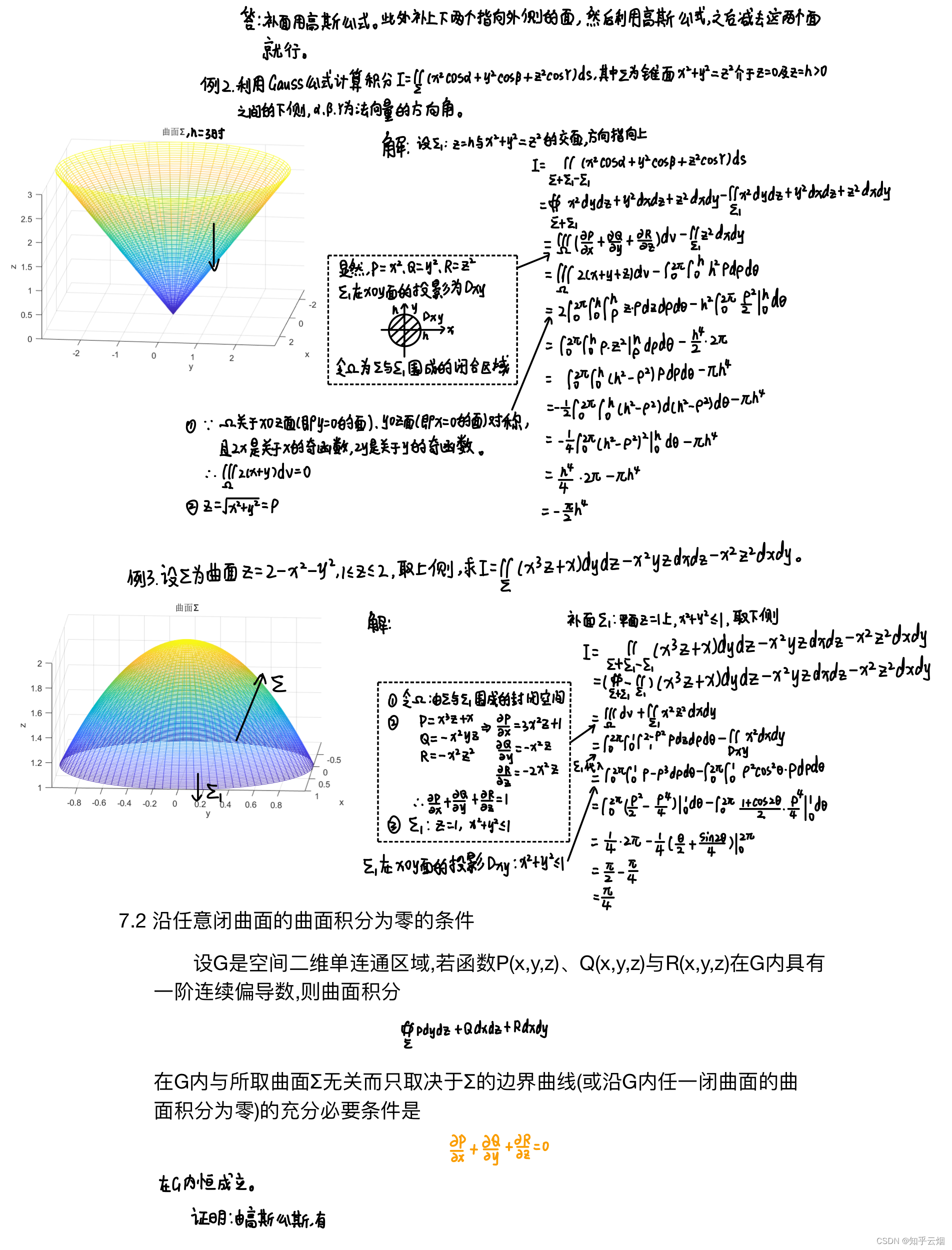
7.1 高斯公式(与格林公式的关系、定义)
7.2 沿任意闭曲面积分的曲面积分为零的条件
例2的代码:
clc;
clear ;
close all;
% 1.曲面Σ的参数方程
h = 3;
theta = linspace(0,2*pi,60);
z = linspace(0,h,80);
[theta,z]=meshgrid(theta,z);
x = sqrt(z.^2).*cos(theta);
y = sqrt(z.^2).*sin(theta);
% 2.画图
figure;
mesh(x,y,z);
hold on;
xlabel('x');
ylabel('y');
zlabel('z');
title('曲面Σ');
grid on;
axis tight;
hidden off %打开透视
hold off;
例3的代码:
clc;
clear ;
close all;
% 1.曲面Σ的参数方程
theta = linspace(0,2*pi,100);
z = linspace(1,2,100);
[theta,z]=meshgrid(theta,z);
x = sqrt(2-z).*cos(theta);
y = sqrt(2-z).*sin(theta);
% 2.画图
figure;
mesh(x,y,z);
hold on;
xlabel('x');
ylabel('y');
zlabel('z');
title('曲面Σ');
grid on;
axis tight;
axis equal;
hidden off %打开透视
hold off;
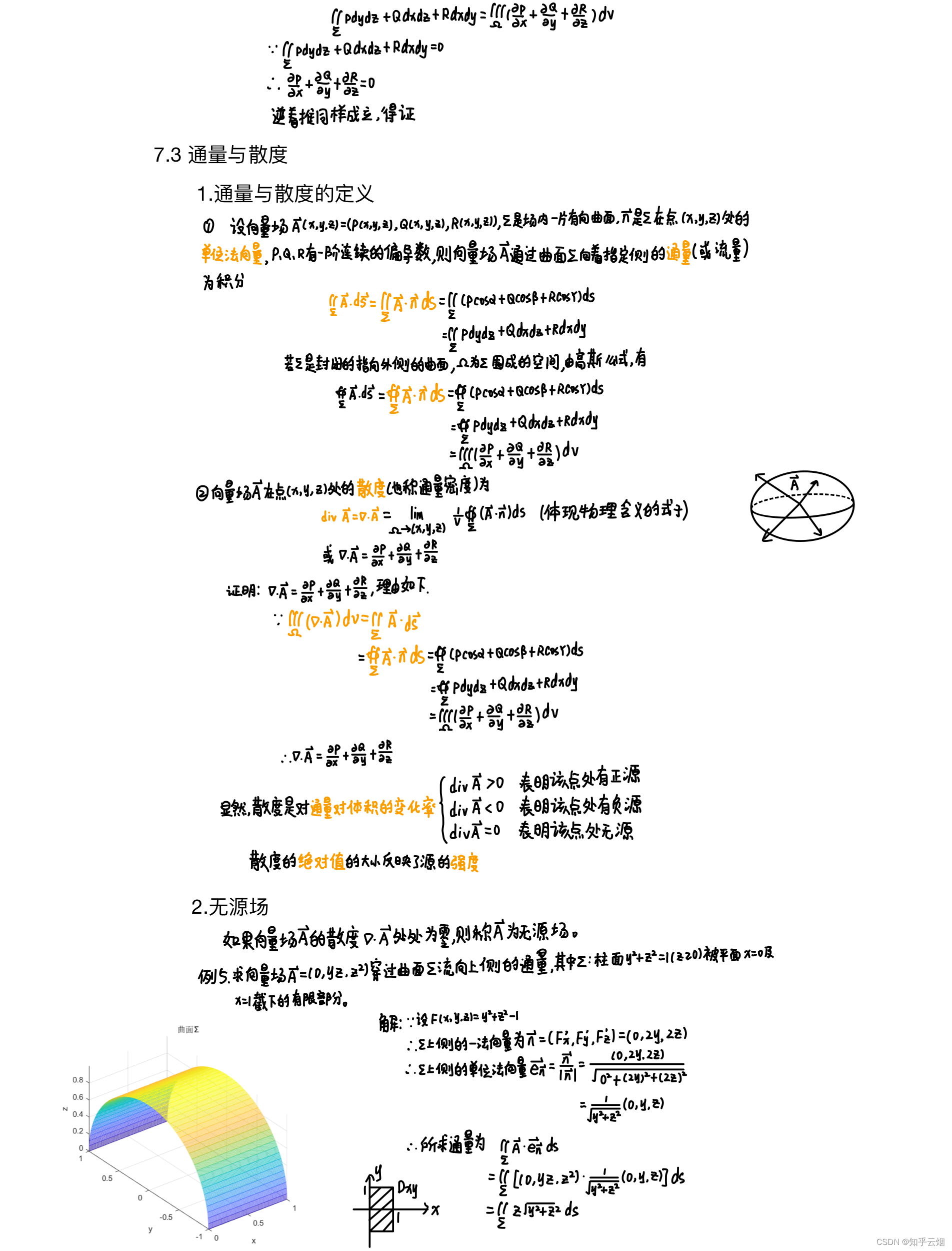
7.3 通量、散度、无源场
例5的代码:
clc;
clear ;
close all;
% 1.曲面Σ的参数方程
theta = linspace(0,pi,50);
x = linspace(0,1,100);
[theta,x]=meshgrid(theta,x);
y = 1.*cos(theta);
z = 1.*sin(theta);
% 2.画图
figure;
mesh(x,y,z);
hold on;
xlabel('x');
ylabel('y');
zlabel('z');
title('曲面Σ');
grid on;
axis tight;
axis equal;
hidden off %打开透视
hold off;
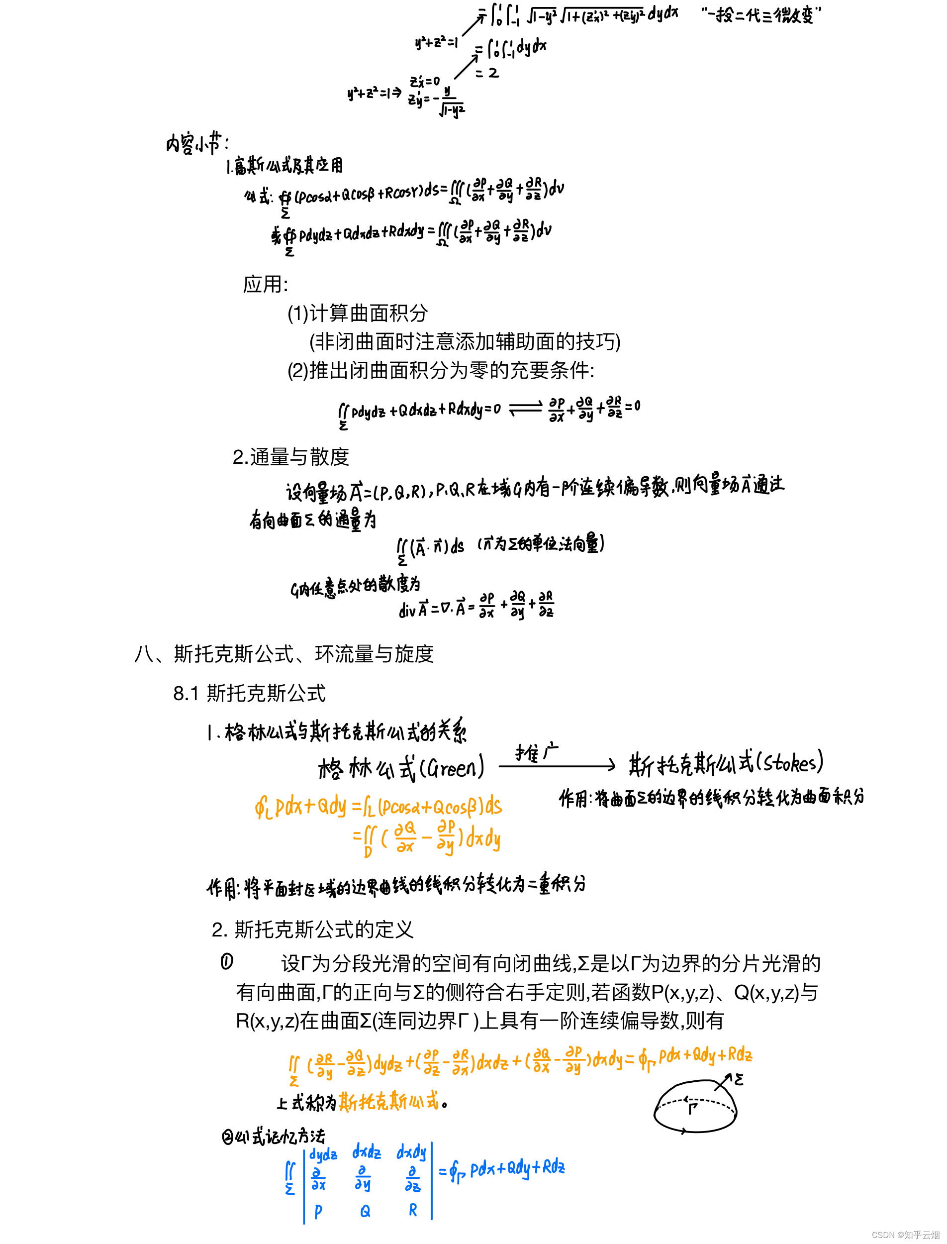
八、斯托克斯公式、环流量与旋度
8.1 斯托克斯公式(与格林公式的关系、定义、证明)
8.2 空间曲线积分与路径无关的条件
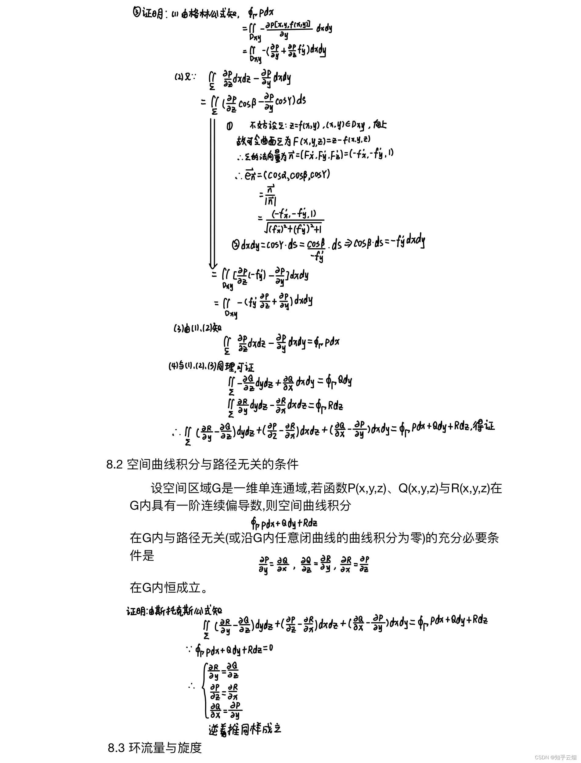
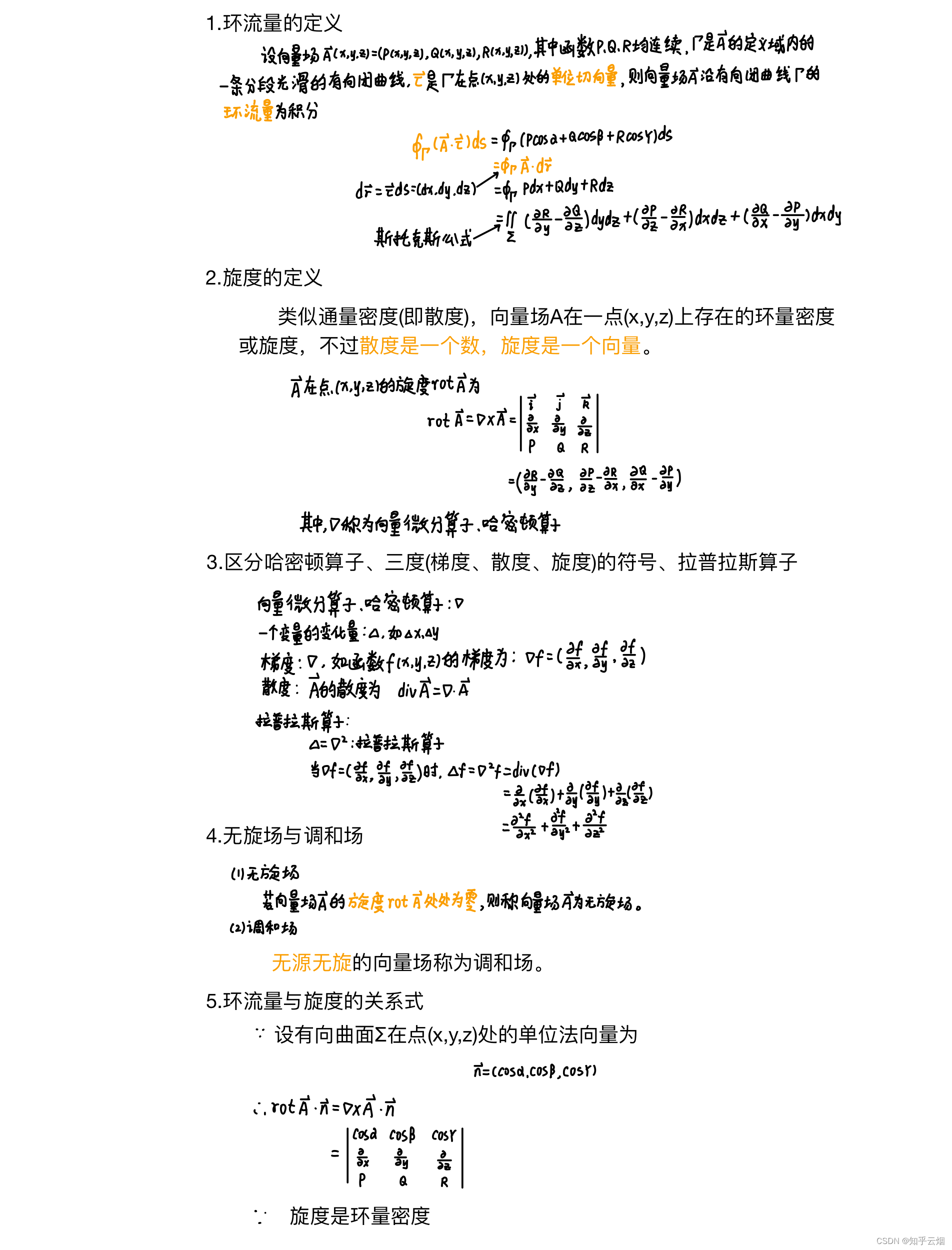
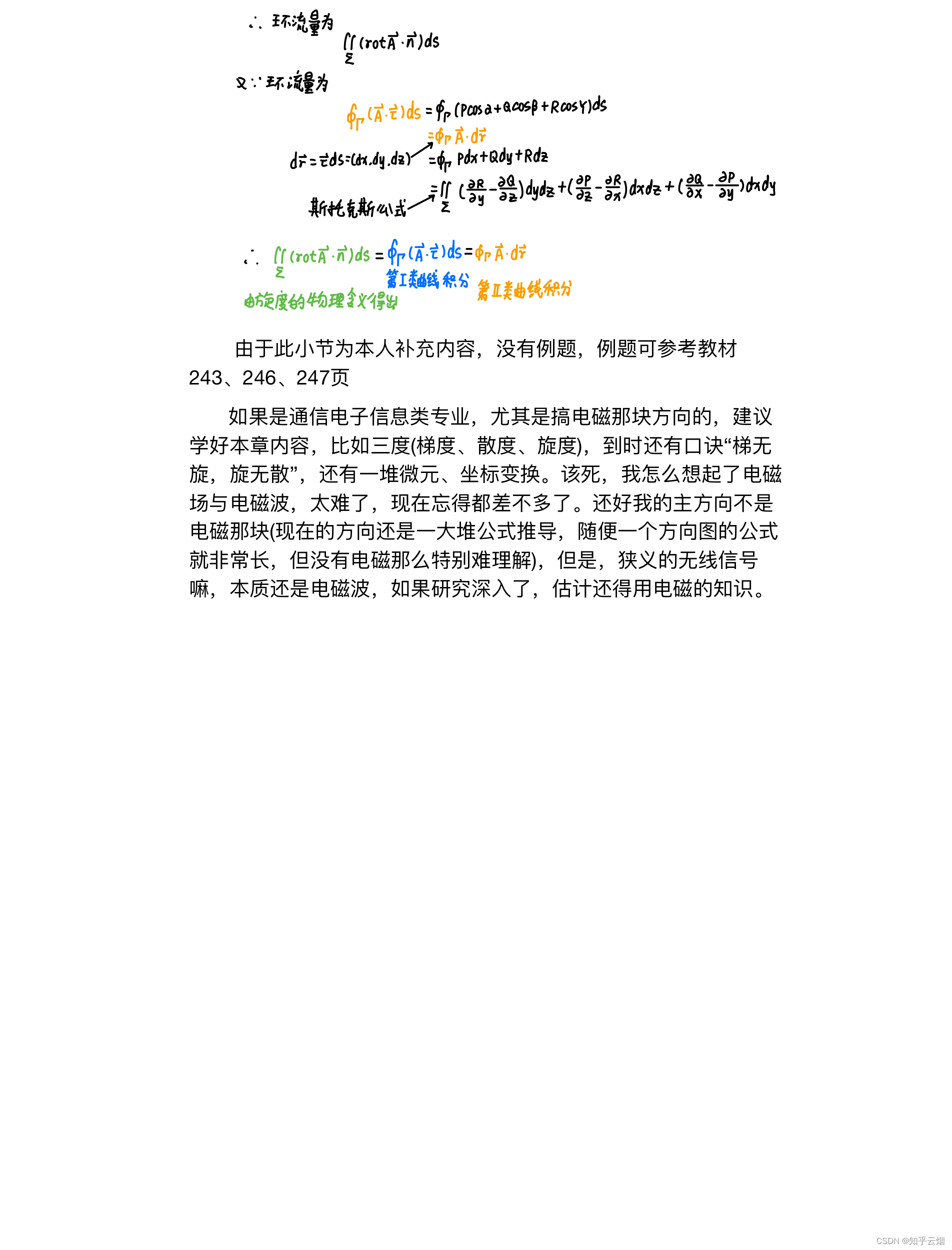
8.3 环流量与旋度(环流量的定义、旋度的定义、几个符号的区分(哈密顿算子、梯度、散度、旋度、拉普拉斯算子)、无旋场与调和场、环流量与旋度的关系式)


 1万+
1万+

 被折叠的 条评论
为什么被折叠?
被折叠的 条评论
为什么被折叠?
 到【灌水乐园】发言


