吴恩达机器学习作业（1）线性回归

一、单变量线性回归

1 导入数据

（1）导入库

import numpy as np
import pandas as pd
import matplotlib.pyplot as plt

（2）导入数据集

data = pd.read_csv('ex1data1.txt',names = ['population','profit'])
data.head()

（3）数据可视化

data.head() #查看前五个
data.tail() #查看后五个
data.describe() #描述性统计
--------------------------------------------------------------
#绘制散点图
data.plot.scatter('population','profit',label = 'population')
plt.show()

2 数据集构建

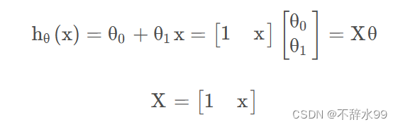
（1）模型选择

根据散点图，选择一元线性回归方程。

（2） X列增加

data.insert(0,'x',1)
data.head()

（3）数据集切割

X = data.iloc[:,0:-1]
X.head()

y = data.iloc[:,-1]
y.head()

（4）数据类型转化与形状查看

X = X.values
X.shape
y = y.values
y.shape

（5）y形状转为二维

y = y.reshape(97,1)
y.shape

3 损失函数

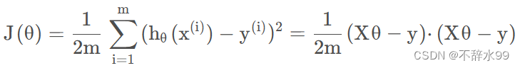
（1）函数定义

def costFunction(X,y,theta):
    inner = np.power(X@theta-y,2)
    return np.sum(inner)/(2*len(X))

 （2）实例化

theta = np.zeros((2,1))
theta.shape
cost_init = costFunction(X,y,theta)
print(cost_init)

4 梯度下降函数

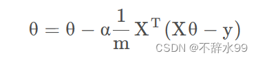
（1）函数定义 

def gradientDescent(X,y,theta,alpha,iters):
    costs = []
    
    for i in range(iters):
        theta = theta - (X.T@(X@theta-y))*alpha/len(X)
        cost = costFunction(X,y,theta)
        costs.append(cost)
        
        if i%100 ==0:
            print(cost)
            
    return theta,costs

 （2）指定学习率与迭代次数，并实例化

alpha=0.02
iters=2000

theta,costs=gradientDescent(X,y,theta,alpha,iters)

5 可视化

fig,ax = plt.subplots()
ax.plot(np.arange(iters),costs)
ax.set(xlabel='iters',
      ylabel='cost',
      title='cost vs iters')
plt.show()

二、多变量线性回归

1 导入数据

（1）导入库

import numpy as np
import pandas as pd
import matplotlib.pyplot as plt

（2）导入数据

data = pd.read_csv('ex1data2.txt',names=['size','bedrooms','price'])
data.head()

（3）特征归一化

def normalize_feature(data):
    return (data-data.mean())/data.std()
data = normalize_feature(data)

（4）可视化

data.plot.scatter('size','price',label='size')
plt.show()

data.plot.scatter('bedrooms','price',label='bedrooms')
plt.show()

2 构造数据集

（1）X列增加

data.insert(0,'x',1)
data.head()

（2）数据集分割

X = data.iloc[:,0:-1]

y = data.iloc[:,-1]

（3）数据类型转化与形状查看

X = X.values
X.shape
y = y.values
y = y.reshape(47,1)

3 损失函数

def costFunction(X,y,theta):
    inner = np.power(X@theta-y,2)
    return np.sum(inner)/(2*len(X))

theta = np.zeros((3,1))

4 梯度下降函数

def gradientDescent(X,y,theta,alpha,iters,isprint=False):
    costs = []
    
    for i in range(iters):
        theta = theta - (X.T @ (X@theta - y) ) * alpha / len(X)
        cost = costFunction(X,y,theta)
        costs.append(cost)
        
        if i%100==0:
            if isprint:
                print(cost)
    
    return theta,costs

5 学习率选择

candinate_alpha = [0.0003,0.003,0.03,0.0001,0.001,0.01]
iters = 2000

fig,ax = plt.subplots()

for alpha in candinate_alpha:
    _,costs=gradientDescent(X,y,theta,alpha,iters)
    ax.plot(np.arange(iters),costs,label = alpha)
    ax.legend()
ax.set(xlabel='iters',
      ylabel='cost',
      title='cost vs iters')
plt.show()