数据挖掘——手写体数字识别

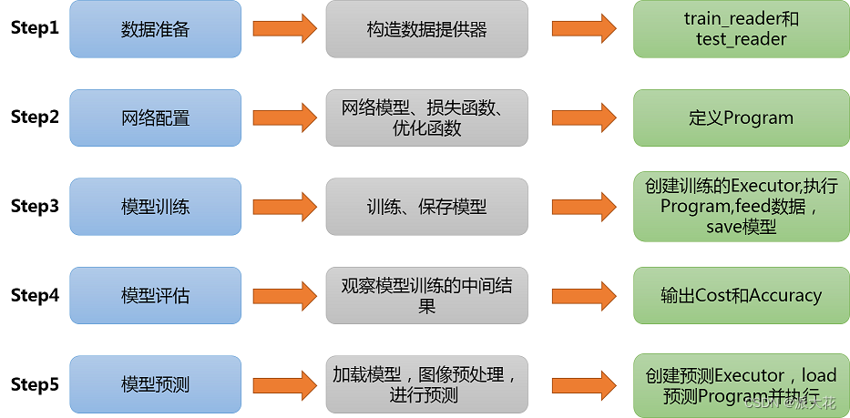
首先导入必要的包：

numpy---------->python第三方库，用于进行科学计算

PIL------------> Python Image Library,python第三方图像处理库

matplotlib----->python的绘图库 pyplot:matplotlib的绘图框架

os------------->提供了丰富的方法来处理文件和目录

#导入需要的包
import numpy as np
import paddle as paddle
import paddle.fluid as fluid
from PIL import Image
import matplotlib.pyplot as plt
import os
from paddle.fluid.dygraph import Linear

Step1：准备数据

（1）数据集介绍

MNIST数据集包含60000个训练集和10000测试数据集。分为图片和标签，图片是28*28的像素矩阵，标签为0~9共10个数字。

（2）train_reader和test_reader

paddle.dataset.mnist.train()和test()分别用于获取mnist训练集和测试集

paddle.batch()表示每BATCH_SIZE组成一个batch

paddle.reader.shuffle()表示每次缓存BUF_SIZE个数据项，并在读取一个数据项前进行随机排序。

（3）打印看下数据是什么样的？PaddlePaddle接口提供的数据已经经过了归一化、居中等处理。

!mkdir -p /home/aistudio/.cache/paddle/dataset/mnist/
!cp -r /home/aistudio/data/data65/*  /home/aistudio/.cache/paddle/dataset/mnist/
!ls /home/aistudio/.cache/paddle/dataset/mnist/

BUF_SIZE=512
BATCH_SIZE=128  #每次流中可以获取的数据量
#用于训练的数据提供器，每次从缓存的数据项中随机读取批次大小的数据
train_reader = paddle.batch(
    paddle.reader.shuffle(paddle.dataset.mnist.train(),
                          buf_size=BUF_SIZE),
    batch_size=BATCH_SIZE)
#用于训练的数据提供器，每次从缓存的数据项中随机读取批次大小的数据
test_reader = paddle.batch(
    paddle.reader.shuffle(paddle.dataset.mnist.test(),
                          buf_size=BUF_SIZE),
    batch_size=BATCH_SIZE)

#用于打印，查看mnist数据
train_data=paddle.dataset.mnist.train();
sampledata=next(train_data())
print(sampledata)

Step2.网络配置

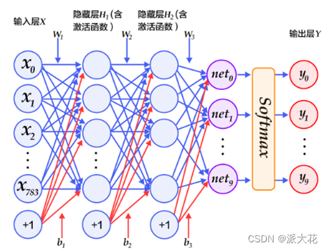
以下的代码判断就是定义一个简单的多层感知器，一共有三层，两个大小为100的隐层和一个大小为10的输出层，因为MNIST数据集是手写0到9的灰度图像，类别有10个，所以最后的输出大小是10。最后输出层的激活函数是Softmax，所以最后的输出层相当于一个分类器。加上一个输入层的话，多层感知器的结构是：输入层-->>隐层-->>隐层-->>输出层。

# 定义多层感知器 
#动态图定义多层感知器
# TO DO：修改网络结构，提升性能
class multilayer_perceptron(fluid.dygraph.Layer):
    def __init__(self):
        super(multilayer_perceptron,self).__init__()    #从父类继承属性
        #输入为28*28的图像，输出该图像的100个特征点，使用relu函数作为激活函数
        #fc1，fc2相当于一个过滤器
        self.fc1 = Linear(input_dim=28*28, output_dim=100, act='relu') 
        self.fc2 = Linear(input_dim=100, output_dim=100, act='relu')
        #最后一层过滤得到的是10*1的概率矩阵，值的大小即为概率的大小，概率最大的值所在下标即是答案
        self.fc3 = Linear(input_dim=100, output_dim=10,act="softmax")
        
    def forward(self,input_):
        x = fluid.layers.reshape(input_, [input_.shape[0], -1])
        x = self.fc1(x)
        x = self.fc2(x)
        y = self.fc3(x)
        return y

展示模型训练曲线。 

all_train_iter=0
all_train_iters=[]
all_train_costs=[]
all_train_accs=[]


#绘制训练过程
def draw_train_process(title,iters,costs,accs,label_cost,lable_acc):
    plt.title(title, fontsize=24)
    plt.xlabel("iter", fontsize=20)
    plt.ylabel("cost/acc", fontsize=20)
    plt.plot(iters, costs,color='red',label=label_cost) 
    plt.plot(iters, accs,color='green',label=lable_acc) 
    plt.legend()
    plt.grid()
    plt.show()


def draw_process(title,color,iters,data,label):
    plt.title(title, fontsize=24)
    plt.xlabel("iter", fontsize=20)
    plt.ylabel(label, fontsize=20)
    plt.plot(iters, data,color=color,label=label) 
    plt.legend()
    plt.grid()
    plt.show()

Step3.模型训练并评估

训练需要有一个训练程序和一些必要参数，并构建了一个获取训练过程中测试误差的函数。必要参数有executor,program,reader,feeder,fetch_list。

#用动态图进行训练
all_train_iter=0
all_train_iters=[]
all_train_costs=[]
all_train_accs=[]

best_test_acc = 0.0


with fluid.dygraph.guard():
    model=multilayer_perceptron() #模型实例化
    model.train() #训练模式
    opt=fluid.optimizer.Adam(learning_rate=fluid.dygraph.ExponentialDecay(
              learning_rate=0.001 ,            decay_steps=4000,
              decay_rate=0.1,
              staircase=True), parameter_list=model.parameters())
    
  
    epochs_num=20 #迭代次数
    #一般来的，跌打次数越多，精度越高
    
    for pass_num in range(epochs_num):
        lr = opt.current_step_lr()
        print("learning-rate:", lr)
        
        for batch_id,data in enumerate(train_reader()):
            
            images=np.array([x[0].reshape(1,28,28) for x in data],np.float32)
            
            labels = np.array([x[1] for x in data]).astype('int64')
            labels = labels[:, np.newaxis]
            
            image=fluid.dygraph.to_variable(images)
            label=fluid.dygraph.to_variable(labels)
            predict=model(image)#预测
            #print(predict)
            loss=fluid.layers.cross_entropy(predict,label)
            avg_loss=fluid.layers.mean(loss)#获取loss值
            
            acc=fluid.layers.accuracy(predict,label)#计算精度
            avg_loss.backward()
            opt.minimize(avg_loss)
            model.clear_gradients()

            all_train_iter=all_train_iter+256
            all_train_iters.append(all_train_iter)
            all_train_costs.append(loss.numpy()[0])
            all_train_accs.append(acc.numpy()[0])
            
            
            if batch_id!=0 and batch_id%50==0:
                print("train_pass:{},batch_id:{},train_loss:{},train_acc:{}".format(pass_num,batch_id,avg_loss.numpy(),acc.numpy()))
        
        
        with fluid.dygraph.guard():
            accs = []
            model.eval()#评估模式
            for batch_id,data in enumerate(test_reader()):#测试集
                images=np.array([x[0].reshape(1,28,28) for x in data],np.float32)
                labels = np.array([x[1] for x in data]).astype('int64')
                labels = labels[:, np.newaxis]
            
                image=fluid.dygraph.to_variable(images)
                label=fluid.dygraph.to_variable(labels)
            
                predict=model(image)#预测
                acc=fluid.layers.accuracy(predict,label)
                accs.append(acc.numpy()[0])
                avg_acc = np.mean(accs)
           
           
            if avg_acc >= best_test_acc:
                best_test_acc = avg_acc
                if pass_num > 10:
                    fluid.save_dygraph(model.state_dict(),'./work/{}'.format(pass_num))#保存模型
            
            print('Test:%d, Accuracy:%0.5f, Best: %0.5f'%  (pass_num, avg_acc, best_test_acc))

            
    fluid.save_dygraph(model.state_dict(),'./work/fashion_mnist_epoch{}'.format(epochs_num))#保存模型


print('训练模型保存完成！')
print("best_test_acc", best_test_acc)
draw_train_process("training",all_train_iters,all_train_costs,all_train_accs,"trainning cost","trainning acc")  
draw_process("trainning loss","red",all_train_iters,all_train_costs,"trainning loss")
draw_process("trainning acc","green",all_train_iters,all_train_accs,"trainning acc")  

Step4.模型预测

（1）图片预处理

在预测之前，要对图像进行预处理。

首先进行灰度化，然后压缩图像大小为28*28，接着将图像转换成一维向量，最后再对一维向量进行归一化处理。

def load_image(file):
    im = Image.open(file).convert('L')                        #将RGB转化为灰度图像，L代表灰度图像，像素值在0~255之间
    im = im.resize((28, 28), Image.ANTIALIAS)                 #resize image with high-quality 图像大小为28*28
    im = np.array(im).reshape(1, 1, 28, 28).astype(np.float32)#返回新形状的数组,把它变成一个 numpy 数组以匹配数据馈送格式。
    print(im)
    im = im / 255.0 * 2.0 - 1.0                               #归一化到【-1~1】之间
    return im

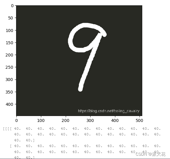
（2）使用Matplotlib工具显示这张图像并预测。

infer_path='/home/aistudio/data/data2304/infer-9.png'
img = Image.open(infer_path)
plt.imshow(img)   #根据数组绘制图像
plt.show()        #显示图像
label_list = [
    "0", "1", "2", "3", "4", "5", "6", "7","8", "9","10"
    ]

#构建预测动态图过程
model_path = './work/11'
with fluid.dygraph.guard():
    model=multilayer_perceptron()#模型实例化
    model_dict,_=fluid.load_dygraph(model_path)
    model.load_dict(model_dict)#加载模型参数
    model.eval()#评估模式
    infer_img = load_image(infer_path)
    infer_img=np.array(infer_img).astype('float32')
    infer_img=infer_img[np.newaxis,:, : ,:]
    infer_img = fluid.dygraph.to_variable(infer_img)
    result=model(infer_img)
   
    print("infer results: %s" % label_list[np.argmax(result.numpy())])

（3）运行部分截图如下：