MeshGraphNets Paddle复现

AI Studio

已于 2023-01-13 20:47:00 修改

阅读量1.1k

点赞数 1

文章标签： paddle 深度学习人工智能

于 2023-01-08 22:34:28 首次发布

原文链接：https://aistudio.baidu.com/aistudio/projectdetail/5372511?forkThirdPart=1

版权

meshgraphnets_paddlepaddle

Github地址：https://github.com/jiamingkong/meshgraphnets_paddlepaddle

1. 简介

本项目旨在用PaddlePaddle框架复现[2010.03409] Learning Mesh-Based Simulation with Graph Networks (arxiv.org) 论文，目前支持了原论文中cylinder_flow数据集的模拟。

1.1 模型设计的动机

简单地说，这个模型学习的是物理模拟的知识。以cylinder_flow数据为例，数据集描述的是水流通过一个带有圆柱形障碍物的通道后产生的绕流情况。在常规的流体力学模拟里面，为了提升计算效率并降低误差，我们往往会使用非匀质的网络（Mesh）对整个场景进行划分。一个典型的划分场景如下：

可以看到我们会选择在流速变动较大的地方（例如柱子边缘，管道边缘）采取更密的点阵，在其他地方采取更疏的点阵，这样一来，计算资源就更有效地分配在精度要求高的地方。但这也引发了一定的问题——我们无法再使用常规的神经网络例如Unet / CNN / Transformer 的结构对非匀质网络进行处理。图网络(graph neural network)天生对这样的网格结构有更好的适应性。所以Deepmind的研究人员就使用了图网络来学习流体力学的模拟知识。

同时，图神经网络高度并行的特性能为物理模拟加速。该项目中成型的模型进行物理模拟的速度，在相同硬件条件上，比传统数值模拟软件快两个数量级。

1.2 模型的输入和输出

在不考虑碰撞等情况下，模型的输入和输出都是一个图G = (V,E)。每个图有多个点 $V_i, V_j, ...$ ，对应上述的划分（Mesh）上的点。同时点之间有边相连 $E_{ij}$ 。每个点和边的信息都是一个向量，具体组成如下：

$V_i$ 的信息：

每个点的类型 $n_i$ ，这个点是边/障碍物/还是水流等
这个点在t-1时刻的物理量（例如速度在xyz轴上的分量，压强等） $w_i$ ，在cylinder_flow的设定里， $w_i$ 是速度分量。

$E_{ij}$ 的信息：

两个点的相对位置 $u_{ij}$
两个点的距离 $u_{ij}|$

模型的输出是：

每个点下一个时刻的物理量的变化量 $\dot{w}_{i}$

这时候我们外推下一个时刻的系统状态，则可以通过 $w_{i, t} = w_{i,t-1} + \dot{w}_{i,t}$ 来进行

1.3 模型的计算逻辑

和很多图神经网络一样，这个MeshGraphNets也采取了Encode-Process-Decode的三步骤。

Encoder

Encoder将每个边和点的信息都映射成128维的特征，具体的实现在model/model.py 中体现。

Processor

Processor将每个点和边的信息聚合后计算，具体的逻辑如下（下面使用的变量都是原始的 $v_i$ , $e_{ij}$ 信息被映射到128维特征后的变量）：

$e'_{ij} = f(e_{ij}, v_i, v_j)$
一个边的下一时刻的128维特征 = f(这个边的当前时刻特征，边的两个端点的特征)，f是一个MLP函数。

$v'_i = f^V(v_i, \sum_j e'_{ij})$

一个点的下一时刻的128维特征 = fv(这个点的当前时刻的特征，与这个点有关的所有边的128维特征的求和), fv也是一个mlp函数。

Decoder

Decoder就是简单地将128维特征映射回每个点/边应有的特征数量。

2. 数据准备

为了aistudio中再现方便，我们准备了一个小型的数据切片（500mb），原始数据h5格式为50gb。我们的训练和可视化的过程都将基于这个切片。

如果要复现完整的项目，请参考github版本。

import os

dataset_dir = "/home/aistudio/data/data184320"
os.listdir(dataset_dir)

['valid.h5']

# 如果需要进行持久化安装, 需要使用持久化路径, 如下方代码示例:
# If a persistence installation is required, 
# you need to use the persistence path as the following: 

!mkdir /home/aistudio/external-libraries
!pip install tqdm opencv_python -t /home/aistudio/external-libraries

# 同时添加如下代码, 这样每次环境(kernel)启动的时候只要运行下方代码即可: 
# Also add the following code, 
# so that every time the environment (kernel) starts, 
# just run the following code: 
import sys 
sys.path.append('/home/aistudio/external-libraries')

3. 训练

使用train.py进行训练，参数格式如下：

python train.py \
  --gpu
  --gpu_id 0
  --model_dir checkpoint/cylinder_flow
  --noise_std 0.02
  --data_dir data/cylinder_flow/datapkls
  --lr 0.0001
  --batch_size 4
  --gradient_accumulation_step 32
  --save_interval 200
  --max_epoch 20

请开启GPU环境，并使用下面cell中代码进行训练。

# ! python train.py --gpu \
#   --gpu_id 0 \
#   --model_dir checkpoint/1.pdparams \
#   --noise_std 0.02 \
#   --data_dir /home/aistudio/data/data184320 \
#   --split valid \
#   --lr 0.0001 \
#   --batch_size 4 \
#   --gradient_accumulation_step 32 \
#   --save_interval 200 \
#   --max_epoch 20

W1227 13:46:40.997643  1183 gpu_resources.cc:61] Please NOTE: device: 0, GPU Compute Capability: 7.0, Driver API Version: 11.2, Runtime API Version: 11.2
W1227 13:46:41.001922  1183 gpu_resources.cc:91] device: 0, cuDNN Version: 8.2.
Simulator model initialized
Dataset /home/aistudio/data/data184320/valid.h5 Initialized
Simulator model loaded checkpoint checkpoint/1.pdparams
All set up, start training
Epoch Finished
Cylinder Flow:0 loss = 0.000 (current = 0.000)
Cylinder Flow:1 loss = 0.006 (current = 0.052)
Cylinder Flow:2 loss = 0.011 (current = 0.059)
Cylinder Flow:3 loss = 0.015 (current = 0.054)
Cylinder Flow:4 loss = 0.019 (current = 0.054)
Cylinder Flow:5 loss = 0.023 (current = 0.053)
Cylinder Flow:6 loss = 0.026 (current = 0.054)
Cylinder Flow:7 loss = 0.029 (current = 0.060)
Cylinder Flow:8 loss = 0.031 (current = 0.053)
Cylinder Flow:9 loss = 0.034 (current = 0.052)
Cylinder Flow:10 loss = 0.036 (current = 0.053)
Cylinder Flow:11 loss = 0.037 (current = 0.050)
Cylinder Flow:12 loss = 0.039 (current = 0.054)
Cylinder Flow:13 loss = 0.040 (current = 0.052)
Cylinder Flow:14 loss = 0.042 (current = 0.056)
Cylinder Flow:15 loss = 0.043 (current = 0.052)
Cylinder Flow:16 loss = 0.044 (current = 0.053)
Cylinder Flow:17 loss = 0.044 (current = 0.051)
Cylinder Flow:18 loss = 0.045 (current = 0.051)
Cylinder Flow:19 loss = 0.046 (current = 0.055)
Cylinder Flow:20 loss = 0.047 (current = 0.053)
Cylinder Flow:21 loss = 0.048 (current = 0.055)
Cylinder Flow:22 loss = 0.048 (current = 0.056)
Cylinder Flow:23 loss = 0.049 (current = 0.051)
Cylinder Flow:24 loss = 0.049 (current = 0.053)
Cylinder Flow:25 loss = 0.049 (current = 0.052)
Cylinder Flow:26 loss = 0.050 (current = 0.053)
Cylinder Flow:27 loss = 0.050 (current = 0.055)
Cylinder Flow:28 loss = 0.051 (current = 0.053)
Cylinder Flow:29 loss = 0.051 (current = 0.051)
Cylinder Flow:30 loss = 0.051 (current = 0.051)
Cylinder Flow:31 loss = 0.051 (current = 0.055)
Cylinder Flow:32 loss = 0.051 (current = 0.051)
Cylinder Flow:33 loss = 0.046 (current = 0.002)
Cylinder Flow:34 loss = 0.042 (current = 0.002)
Cylinder Flow:35 loss = 0.038 (current = 0.002)
Cylinder Flow:36 loss = 0.034 (current = 0.003)
Cylinder Flow:37 loss = 0.031 (current = 0.002)
Cylinder Flow:38 loss = 0.029 (current = 0.004)
Cylinder Flow:39 loss = 0.026 (current = 0.003)
Cylinder Flow:40 loss = 0.024 (current = 0.003)
Cylinder Flow:41 loss = 0.021 (current = 0.003)
Cylinder Flow:42 loss = 0.020 (current = 0.003)
Cylinder Flow:43 loss = 0.018 (current = 0.002)
Cylinder Flow:44 loss = 0.016 (current = 0.002)
Cylinder Flow:45 loss = 0.015 (current = 0.003)
Cylinder Flow:46 loss = 0.014 (current = 0.003)
Cylinder Flow:47 loss = 0.013 (current = 0.004)
Cylinder Flow:48 loss = 0.012 (current = 0.003)
Cylinder Flow:49 loss = 0.011 (current = 0.003)
Cylinder Flow:50 loss = 0.010 (current = 0.003)
Cylinder Flow:51 loss = 0.009 (current = 0.003)
Cylinder Flow:52 loss = 0.009 (current = 0.004)
Cylinder Flow:53 loss = 0.008 (current = 0.003)
Cylinder Flow:54 loss = 0.008 (current = 0.003)
Cylinder Flow:55 loss = 0.007 (current = 0.004)
Cylinder Flow:56 loss = 0.007 (current = 0.003)
Cylinder Flow:57 loss = 0.006 (current = 0.003)
Cylinder Flow:58 loss = 0.006 (current = 0.003)
Cylinder Flow:59 loss = 0.006 (current = 0.003)
Cylinder Flow:60 loss = 0.005 (current = 0.002)
Cylinder Flow:61 loss = 0.005 (current = 0.003)
Cylinder Flow:62 loss = 0.005 (current = 0.002)
Cylinder Flow:63 loss = 0.005 (current = 0.003)
Cylinder Flow:64 loss = 0.004 (current = 0.002)
Cylinder Flow:65 loss = 0.005 (current = 0.015)
Cylinder Flow:66 loss = 0.006 (current = 0.014)
Cylinder Flow:67 loss = 0.007 (current = 0.015)
Cylinder Flow:68 loss = 0.008 (current = 0.015)
Cylinder Flow:69 loss = 0.009 (current = 0.016)
Cylinder Flow:70 loss = 0.009 (current = 0.015)
Cylinder Flow:71 loss = 0.010 (current = 0.015)
Cylinder Flow:72 loss = 0.010 (current = 0.015)
Cylinder Flow:73 loss = 0.011 (current = 0.016)
Cylinder Flow:74 loss = 0.011 (current = 0.015)
Cylinder Flow:75 loss = 0.012 (current = 0.014)
Cylinder Flow:76 loss = 0.012 (current = 0.015)
Cylinder Flow:77 loss = 0.012 (current = 0.014)
Cylinder Flow:78 loss = 0.012 (current = 0.014)
Cylinder Flow:79 loss = 0.013 (current = 0.014)
Cylinder Flow:80 loss = 0.013 (current = 0.015)
Cylinder Flow:81 loss = 0.013 (current = 0.014)
Cylinder Flow:82 loss = 0.013 (current = 0.015)
Cylinder Flow:83 loss = 0.013 (current = 0.016)
Cylinder Flow:84 loss = 0.014 (current = 0.016)
Cylinder Flow:85 loss = 0.014 (current = 0.016)
Cylinder Flow:86 loss = 0.014 (current = 0.014)
Cylinder Flow:87 loss = 0.014 (current = 0.015)
Cylinder Flow:88 loss = 0.014 (current = 0.016)
Cylinder Flow:89 loss = 0.014 (current = 0.014)
Cylinder Flow:90 loss = 0.014 (current = 0.015)
Cylinder Flow:91 loss = 0.014 (current = 0.014)
Cylinder Flow:92 loss = 0.014 (current = 0.015)
Cylinder Flow:93 loss = 0.014 (current = 0.015)
Cylinder Flow:94 loss = 0.014 (current = 0.014)
Cylinder Flow:95 loss = 0.014 (current = 0.015)
Cylinder Flow:96 loss = 0.014 (current = 0.016)
Cylinder Flow:97 loss = 0.014 (current = 0.011)
Cylinder Flow:98 loss = 0.014 (current = 0.009)
Cylinder Flow:99 loss = 0.013 (current = 0.009)
Cylinder Flow:100 loss = 0.013 (current = 0.010)
Cylinder Flow:101 loss = 0.013 (current = 0.009)
Cylinder Flow:102 loss = 0.012 (current = 0.010)
Cylinder Flow:103 loss = 0.012 (current = 0.010)
Cylinder Flow:104 loss = 0.012 (current = 0.010)
Cylinder Flow:105 loss = 0.012 (current = 0.009)
Cylinder Flow:106 loss = 0.011 (current = 0.010)
Cylinder Flow:107 loss = 0.011 (current = 0.010)
Cylinder Flow:108 loss = 0.011 (current = 0.009)
Cylinder Flow:109 loss = 0.011 (current = 0.009)
Cylinder Flow:110 loss = 0.011 (current = 0.011)
Cylinder Flow:111 loss = 0.011 (current = 0.009)
Cylinder Flow:112 loss = 0.011 (current = 0.010)
Cylinder Flow:113 loss = 0.010 (current = 0.009)
Cylinder Flow:114 loss = 0.010 (current = 0.009)
Cylinder Flow:115 loss = 0.010 (current = 0.009)
Cylinder Flow:116 loss = 0.010 (current = 0.010)
Cylinder Flow:117 loss = 0.010 (current = 0.010)
Cylinder Flow:118 loss = 0.010 (current = 0.010)
Cylinder Flow:119 loss = 0.010 (current = 0.009)
Cylinder Flow:120 loss = 0.010 (current = 0.010)
Cylinder Flow:121 loss = 0.010 (current = 0.009)
Cylinder Flow:122 loss = 0.010 (current = 0.011)
Cylinder Flow:123 loss = 0.010 (current = 0.009)
Cylinder Flow:124 loss = 0.010 (current = 0.010)
Cylinder Flow:125 loss = 0.010 (current = 0.010)
Cylinder Flow:126 loss = 0.010 (current = 0.010)
Cylinder Flow:127 loss = 0.010 (current = 0.010)
Cylinder Flow:128 loss = 0.010 (current = 0.010)
Cylinder Flow:129 loss = 0.009 (current = 0.004)
Cylinder Flow:130 loss = 0.009 (current = 0.004)
Cylinder Flow:131 loss = 0.008 (current = 0.004)
Cylinder Flow:132 loss = 0.008 (current = 0.005)
Cylinder Flow:133 loss = 0.008 (current = 0.004)
Cylinder Flow:134 loss = 0.007 (current = 0.006)
Cylinder Flow:135 loss = 0.007 (current = 0.005)
Cylinder Flow:136 loss = 0.007 (current = 0.006)
Cylinder Flow:137 loss = 0.007 (current = 0.004)
Cylinder Flow:138 loss = 0.007 (current = 0.004)
Cylinder Flow:139 loss = 0.006 (current = 0.004)
Cylinder Flow:140 loss = 0.006 (current = 0.004)
Cylinder Flow:141 loss = 0.006 (current = 0.004)
Cylinder Flow:142 loss = 0.006 (current = 0.004)
Cylinder Flow:143 loss = 0.006 (current = 0.005)
Cylinder Flow:144 loss = 0.005 (current = 0.004)
Cylinder Flow:145 loss = 0.005 (current = 0.005)
Cylinder Flow:146 loss = 0.005 (current = 0.005)
Cylinder Flow:147 loss = 0.005 (current = 0.004)
Cylinder Flow:148 loss = 0.005 (current = 0.006)
Cylinder Flow:149 loss = 0.005 (current = 0.004)
Cylinder Flow:150 loss = 0.005 (current = 0.005)
Cylinder Flow:151 loss = 0.005 (current = 0.004)
Cylinder Flow:152 loss = 0.005 (current = 0.005)
Cylinder Flow:153 loss = 0.005 (current = 0.004)
Cylinder Flow:154 loss = 0.005 (current = 0.005)
Cylinder Flow:155 loss = 0.005 (current = 0.005)
Cylinder Flow:156 loss = 0.005 (current = 0.004)
Cylinder Flow:157 loss = 0.005 (current = 0.006)
Cylinder Flow:158 loss = 0.005 (current = 0.005)
Cylinder Flow:159 loss = 0.005 (current = 0.005)
^C
Traceback (most recent call last):
  File "train.py", line 90, in <module>
    loss.backward()
  File "<decorator-gen-157>", line 2, in backward
  File "/opt/conda/envs/python35-paddle120-env/lib/python3.7/site-packages/paddle/fluid/wrapped_decorator.py", line 26, in __impl__
    return wrapped_func(*args, **kwargs)
  File "/opt/conda/envs/python35-paddle120-env/lib/python3.7/site-packages/paddle/fluid/framework.py", line 534, in __impl__
    return func(*args, **kwargs)
  File "/opt/conda/envs/python35-paddle120-env/lib/python3.7/site-packages/paddle/fluid/dygraph/varbase_patch_methods.py", line 297, in backward
    core.eager.run_backward([self], grad_tensor, retain_graph)
KeyboardInterrupt

训练的结果会保存在/home/aistudio/checkpoint/下面，其中checkpoing/1.pdparam 是已经训练好的绕流模型。

4. 推理

4.1 计算网格结果

模型训练后进行推理可以使用rollout.py：

python rollout.py \
  --gpu \
  --rollout_num 3 \
  --model_dir checkpoint/cylinder_flow \
  --data_dir data/cylinder_flow/datapkls

在result/文件夹中会输出多个pkl文件，记录测试集的外推结果。

! python rollout.py \
  --gpu \
  --rollout_num 3 \
  --model_dir checkpoint/1.pdparams \
  --data_dir /home/aistudio/data/data184320 \
  --test_split valid

W1227 13:55:04.007498  2899 gpu_resources.cc:61] Please NOTE: device: 0, GPU Compute Capability: 7.0, Driver API Version: 11.2, Runtime API Version: 11.2
W1227 13:55:04.011941  2899 gpu_resources.cc:91] device: 0, cuDNN Version: 8.2.
Simulator model initialized
Simulator model loaded checkpoint checkpoint/1.pdparams
100%|████████████████████████████████████████▉| 599/600 [00:16<00:00, 37.22it/s]
------------------------------------------------------------------
testing rmse  @ step 0 loss: 1.87e-03
testing rmse  @ step 50 loss: 5.12e-03
testing rmse  @ step 100 loss: 6.44e-03
testing rmse  @ step 150 loss: 8.47e-03
testing rmse  @ step 200 loss: 1.13e-02
testing rmse  @ step 250 loss: 1.35e-02
testing rmse  @ step 300 loss: 1.51e-02
testing rmse  @ step 350 loss: 1.65e-02
testing rmse  @ step 400 loss: 1.78e-02
testing rmse  @ step 450 loss: 1.90e-02
testing rmse  @ step 500 loss: 2.03e-02
testing rmse  @ step 550 loss: 2.14e-02
100%|████████████████████████████████████████▉| 599/600 [00:15<00:00, 37.70it/s]
------------------------------------------------------------------
testing rmse  @ step 0 loss: 1.84e-03
testing rmse  @ step 50 loss: 6.11e-03
testing rmse  @ step 100 loss: 9.62e-03
testing rmse  @ step 150 loss: 1.26e-02
testing rmse  @ step 200 loss: 1.63e-02
testing rmse  @ step 250 loss: 2.00e-02
testing rmse  @ step 300 loss: 2.22e-02
testing rmse  @ step 350 loss: 2.35e-02
testing rmse  @ step 400 loss: 2.48e-02
testing rmse  @ step 450 loss: 2.65e-02
testing rmse  @ step 500 loss: 2.84e-02
testing rmse  @ step 550 loss: 3.05e-02
100%|████████████████████████████████████████▉| 599/600 [00:15<00:00, 37.45it/s]
------------------------------------------------------------------
testing rmse  @ step 0 loss: 2.07e-03
testing rmse  @ step 50 loss: 5.11e-03
testing rmse  @ step 100 loss: 7.46e-03
testing rmse  @ step 150 loss: 1.05e-02
testing rmse  @ step 200 loss: 1.34e-02
testing rmse  @ step 250 loss: 1.66e-02
testing rmse  @ step 300 loss: 1.99e-02
testing rmse  @ step 350 loss: 2.34e-02
testing rmse  @ step 400 loss: 2.74e-02
testing rmse  @ step 450 loss: 3.15e-02
testing rmse  @ step 500 loss: 3.55e-02
testing rmse  @ step 550 loss: 3.93e-02
------------------------------------------------------------------
testing rmse  @ step 0 loss: 1.93e-03 +- 1.01e-04
testing rmse  @ step 50 loss: 5.45e-03 +- 4.72e-04
testing rmse  @ step 100 loss: 7.84e-03 +- 1.33e-03
testing rmse  @ step 150 loss: 1.05e-02 +- 1.68e-03
testing rmse  @ step 200 loss: 1.37e-02 +- 2.04e-03
testing rmse  @ step 250 loss: 1.67e-02 +- 2.65e-03
testing rmse  @ step 300 loss: 1.91e-02 +- 2.95e-03
testing rmse  @ step 350 loss: 2.11e-02 +- 3.28e-03
testing rmse  @ step 400 loss: 2.33e-02 +- 4.06e-03
testing rmse  @ step 450 loss: 2.57e-02 +- 5.11e-03
testing rmse  @ step 500 loss: 2.81e-02 +- 6.23e-03
testing rmse  @ step 550 loss: 3.04e-02 +- 7.28e-03

4.2 可视化

python visualize_cylinder_flow.py

这个脚本会将result下的pkl都渲染成video文件夹中的mp4视频文件以便可视化。视频中上半部分是参考结果（来自数值计算软件），下半部分是网络结果。

! python visualize_cylinder_flow.py

OpenCV: FFMPEG: tag 0x44495658/'XVID' is not supported with codec id 12 and format 'mp4 / MP4 (MPEG-4 Part 14)'
OpenCV: FFMPEG: fallback to use tag 0x7634706d/'mp4v'
599it [00:46, 13.02it/s]                                                        
video videos/output0.mp4 saved
OpenCV: FFMPEG: tag 0x44495658/'XVID' is not supported with codec id 12 and format 'mp4 / MP4 (MPEG-4 Part 14)'
OpenCV: FFMPEG: fallback to use tag 0x7634706d/'mp4v'
 16%|██████▋                                   | 19/120 [00:07<00:37,  2.70it/s]^C
 16%|██████▋                                   | 19/120 [00:07<00:38,  2.65it/s]
Traceback (most recent call last):
  File "visualize_cylinder_flow.py", line 93, in <module>
    render(i)
  File "visualize_cylinder_flow.py", line 76, in render
    handle1 = axes[0].tripcolor(triang, target_v, vmax=v_max, vmin=v_min)
  File "/opt/conda/envs/python35-paddle120-env/lib/python3.7/site-packages/matplotlib/axes/_axes.py", line 8148, in tripcolor
    return mtri.tripcolor(self, *args, **kwargs)
  File "/opt/conda/envs/python35-paddle120-env/lib/python3.7/site-packages/matplotlib/tri/tripcolor.py", line 132, in tripcolor
    collection = PolyCollection(verts, **kwargs)
  File "/opt/conda/envs/python35-paddle120-env/lib/python3.7/site-packages/matplotlib/collections.py", line 963, in __init__
    self.set_verts(verts, closed)
  File "/opt/conda/envs/python35-paddle120-env/lib/python3.7/site-packages/matplotlib/collections.py", line 984, in set_verts
    self._paths.append(mpath.Path(xy, codes))
  File "/opt/conda/envs/python35-paddle120-env/lib/python3.7/site-packages/matplotlib/path.py", line 139, in __init__
    if (codes.ndim != 1) or len(codes) != len(vertices):
KeyboardInterrupt

5. Paddle复现心得

本项目是基于echowve/meshGraphNets_pytorch: PyTorch implementations of Learning Mesh-based Simulation With Graph Networks (github.com)的paddle重构。

5.1 网络数据的表示和成批

Pytorch对图神经网络支持力度明显好于百度飞桨。其中torch_geometric / torch_scatter等包在构图上非常方便。为了重现这种方便，我们针对这个项目自己重现了torch_geometric中的data项，具体实现在dataset/data.py中。

图数据最有用的一个特性是成批训练(batching)。图网络的成批训练和图像、音频等数据简单的堆叠不同，图网络数据的成批是将多个图拼合成一个大图（这个大图中有多个互不相连的子图），在送入网络中进行推理。所以我们设计了一个函数Data.offset_by_n(n)：

class Data(object):
    def offset_by_n(self, n):
        if self.edge_index is not None:
            self.edge_index = self.edge_index + n
        if self.face is not None:
            self.face = self.face + n
        return self

假设我们有两个图要成批，图一有两个点，图二在拼接上去前，可以方便地把自己的点的ID都加上2，避免和图一重合。

对应的Collator类则在dataloader中发挥作用，将一个批次中的图拼合成大图：

class Collator(object):
    def __call__(self, batch_data):
        """
        batch_data is a list of Data, the collate_fn will produce one big graph with several disconnected subgraphs
        """
        offset = [i.num_nodes for i in batch_data]
        offset = np.cumsum(offset)
        offset = np.insert(offset, 0, 0)
        offset = offset[:-1]
        batch_data = [i.offset_by_n(n) for i, n in zip(batch_data, offset)]

        return Data(
            x=concat([i.x for i in batch_data], axis=0),
            face=concat([i.face for i in batch_data], axis=1),
            y=concat([i.y for i in batch_data], axis=0),
            pos=concat([i.pos for i in batch_data], axis=0),
            edge_index=concat([i.edge_index for i in batch_data], axis=1),
            edge_attr=concat([i.edge_attr for i in batch_data], axis=0),
        )

5.2 稀疏操作

torch_scatter中有一个很方便完成稀疏累加的函数scatter_add，其使用场景通常是将图上一个点的特征与这个点的邻居的特征相加，参考：Scatter — pytorch_scatter 2.1.0 documentation (pytorch-scatter.readthedocs.io)

paddle中相应的实现是：

def scatter_add(src, index, dim_size=None):
    if dim_size is None:
        dim_size = paddle.max(index) + 1

    indices = paddle.unsqueeze(index, axis=1)
    x = paddle.zeros_like(src)
    y = paddle.scatter_nd_add(x, indices, src)
    return y[:dim_size]

一个简单的例子是：

import paddle
from transforms.scatter import scatter_add
x = paddle.arange(1,11)
index = paddle.to_tensor([0,0,0,1,1,1,2,2,2,3])
scatter_add(x, index)

# >> Tensor([6 , 15, 24, 10])

这里面的意思是：将x中前三项求和，放到结果的第0位置，将第四到第六项求和，放到结果的第1位置，如此类推。所以结果的第一项是1+2+3 = 6，第二项是4+5=6 = 15,第三项是7+8+9=24，第四项是10。

5.3 数据变换

一些常用的torch_geometric中的Transformations也被改写成paddle，置入了transforms。在train.py中，我们定义原始图数据的变换只需要这样：

transforms = Compose([FaceToEdge(), Cartesian(norm=False), Distance(norm=False),])

graph = transforms(graph)

6 一些代码细节

我们补充了代码细节一章以便大家修改该模型匹配自己的数据。

6.1 数据库格式是怎么样的？

我们直接可视化其中一些数据进行说明。在train.py中有加载数据的样例：

from dataset import FPC, Data, Collator, DataLoader
from transforms import FaceToEdge, Cartesian, Distance, Compose

train_dataset = FPC(2, "data/data184320", split="valid", small_open_tra_num=10)

one_frame = next(iter(train_dataset))

Dataset data/data184320/valid.h5 Initialized
Epoch Finished

一帧数据有什么？

其中一帧数据包含了如下内容：

Data(
   x:   每个点的信息（参考上面输入的内容，速度分量（x,y)、点的类型（one hot encoding成三列了，共五列)
   pos:  每个点的位置
   y:   每个点上我们要计算的物理量（在这里是x,y轴的速度分量）
   face: 三角形面的描述（每个面的三个顶点的点ID，对应x / pos / y 里面的第一个下标
)

在我们抽取的one_frame里面，我们有1800个点，3500个面：

one_frame

Data(x=[1876, 5], face=[3, 3518], y=[1876, 2], pos=[1876, 2], )

one_frame.face[:, -10]

Tensor(shape=[3], dtype=int64, place=Place(cpu), stop_gradient=True,
       [1464, 1458, 1862])

one_frame.pos[[1464,1458,1862]]

Tensor(shape=[3, 2], dtype=float32, place=Place(cpu), stop_gradient=True,
       [[1.50804603, 0.00899134],
        [1.48965514, 0.00909127],
        [1.48965514, 0.00413240]])

可见其中一个面有三个点，分别是1464号，1458号，以及1862号。它们的坐标也很接近，确实是一个mesh中的面

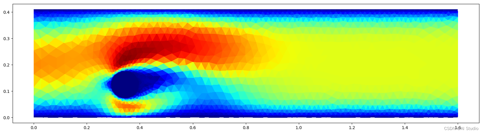
可视化一帧数据

我们现在尝试把一帧数据给画出来：

import matplotlib.tri as tri
import matplotlib.pyplot as plt
import numpy as np
fig, ax = plt.subplots(figsize=(20,10))
ax.set_aspect("equal")
coords = one_frame.pos.numpy()
# 快速转换成三角形
triangles = tri.Triangulation(coords[:,0], coords[:,1])
# 计算每个三角形里的速度分量
velocity = np.linalg.norm(one_frame.y, axis=1)
v_max = np.max(velocity)
v_min = np.min(velocity)
# 绘制三角形
ax.tripcolor(triangles, velocity, vmax=v_max, vmin=v_min, cmap="jet")
plt.show()

在这里插入图片描述

6.2 方便的变换函数

在本项目里我们集成了一些常用的变换函数，方便我们将原始的pos / x 等信息变成实际的embedding:

# 定义变换
transforms = Compose([FaceToEdge(), Cartesian(norm=False), Distance(norm=False),])

# 变换给定的frame
transformed_frame = transforms(one_frame)

print(transformed_frame)

Data(x=[1876, 5], y=[1876, 2], pos=[1876, 2], edge_index=[2, 10788], edge_attr=[10788, 3])

# 定义变换
transforms = Compose([FaceToEdge(), Cartesian(norm=False), Distance(norm=False),])

# 变换给定的frame
transformed_frame = transforms(one_frame)

print(transformed_frame)

Data(x=[1876, 5], y=[1876, 2], pos=[1876, 2], edge_index=[2, 10788], edge_attr=[10788, 3])

可以看到，face被展开成了edge_index（每个面的三个边被拆出来写了），同时每个边都带有了自己的属性（包括相对位移等）。

6.3 数据增强和训练策略

加噪

按照原论文，我们在训练中给每个点的速度分量都加入了噪音。这样能有效防止模型过拟合。

训练策略

有时候我们会发现loss再也下不去，没关系，停下来，把lr再调小一半，继续训练，发现又能下去了。当然使用LR Scheduler也是可以的。

其他探索

把模型中的relu改成gelu，elu，swish效果都不如预期。或许这个物理模拟的过程里并不需要这么多非线性。
模型层数加深比加宽来得有收益，在更大的gpu上，可以考虑把模型层数设定到18，能比起当前模型得出更低误差。

此文章为搬运
原项目链接