识别手写数字（0-9）的深度学习模型

1.直接下载mnist.npz

# 导入所需的库  
import tensorflow as tf  
import numpy as np  
import matplotlib.pyplot as plt  
  
# 加载MNIST数据集，分为训练集和测试集  
# x_train/y_train 是训练集的图片和标签  
# x_test/y_test 是测试集的图片和标签  
(x_train, y_train), (x_test, y_test) = tf.keras.datasets.mnist.load_data()  
  
# 查看第一张图片的形状，MNIST图片是28x28像素的灰度图  
image = x_train[1]  
print(image.shape)  # 输出应该是 (28, 28)  
  
# 取消注释以下两行可以查看第一张图片  
# plt.imshow(image, cmap='gray')  # 使用灰度图模式显示  
# plt.show()  
  
# 取消注释以下一行可以查看第一张图片对应的标签（数字）  
# print(y_train[1])  
  
# 将标签转换为one-hot编码，用于分类任务  
# 例如，数字5将被转换为 [0, 0, 0, 0, 0, 1, 0, 0, 0, 0]  
y_train_one_hot = tf.one_hot(y_train, 10)  
  
# 取消注释以下三行可以查看one-hot编码后的形状、原始训练集形状和第一张图片的one-hot编码  
# print(y_train_one_hot.shape)  
# print(x_train.shape)  
# print(y_train_one_hot[1])  
  
# 定义一个Sequential模型  
model = tf.keras.Sequential([  
    # 将28x28的图片展平为一维向量  
    tf.keras.layers.Flatten(),  
    # 添加一个全连接层，有128个神经元，使用ReLU激活函数  
    tf.keras.layers.Dense(128, activation="relu"),  
    # 再添加两个全连接层，分别有64和32个神经元，都使用ReLU激活函数  
    tf.keras.layers.Dense(64, activation="relu"),  
    tf.keras.layers.Dense(32, activation="relu"),  
    # 注意：这里通常不需要一个18个神经元的层，除非有特别的理由。这里可能是个错误，通常我们会直接连接到输出层  
    # 但为了保持代码的一致性，我保留了这个层  
    tf.keras.layers.Dense(18, activation="relu"),  
    # 输出层，10个神经元对应10个类别，使用softmax激活函数进行多分类  
    tf.keras.layers.Dense(10, activation="softmax"),  
])  
  
# 构建模型，指定输入的形状为 (None, 28, 28)，其中None表示批次大小可以是任意的  
model.build(input_shape=(None, 28, 28))  
  
# 打印模型的结构摘要  
model.summary()  
  
# 编译模型，指定优化器、损失函数和评估指标  
# 注意：这里使用了两个CategoricalCrossentropy，通常我们只需要一个作为损失函数，另一个可以替换为accuracy作为评估指标  
model.compile(optimizer=tf.keras.optimizers.Adam(),   
              loss=tf.keras.losses.CategoricalCrossentropy(),   
              metrics=[tf.keras.metrics.Accuracy()])  # 修改为Accuracy作为评估指标  
  
# 训练模型，使用训练集的图片和one-hot编码的标签，训练10个epoch  
history = model.fit(x_train, y_train_one_hot, epochs=10)  
  
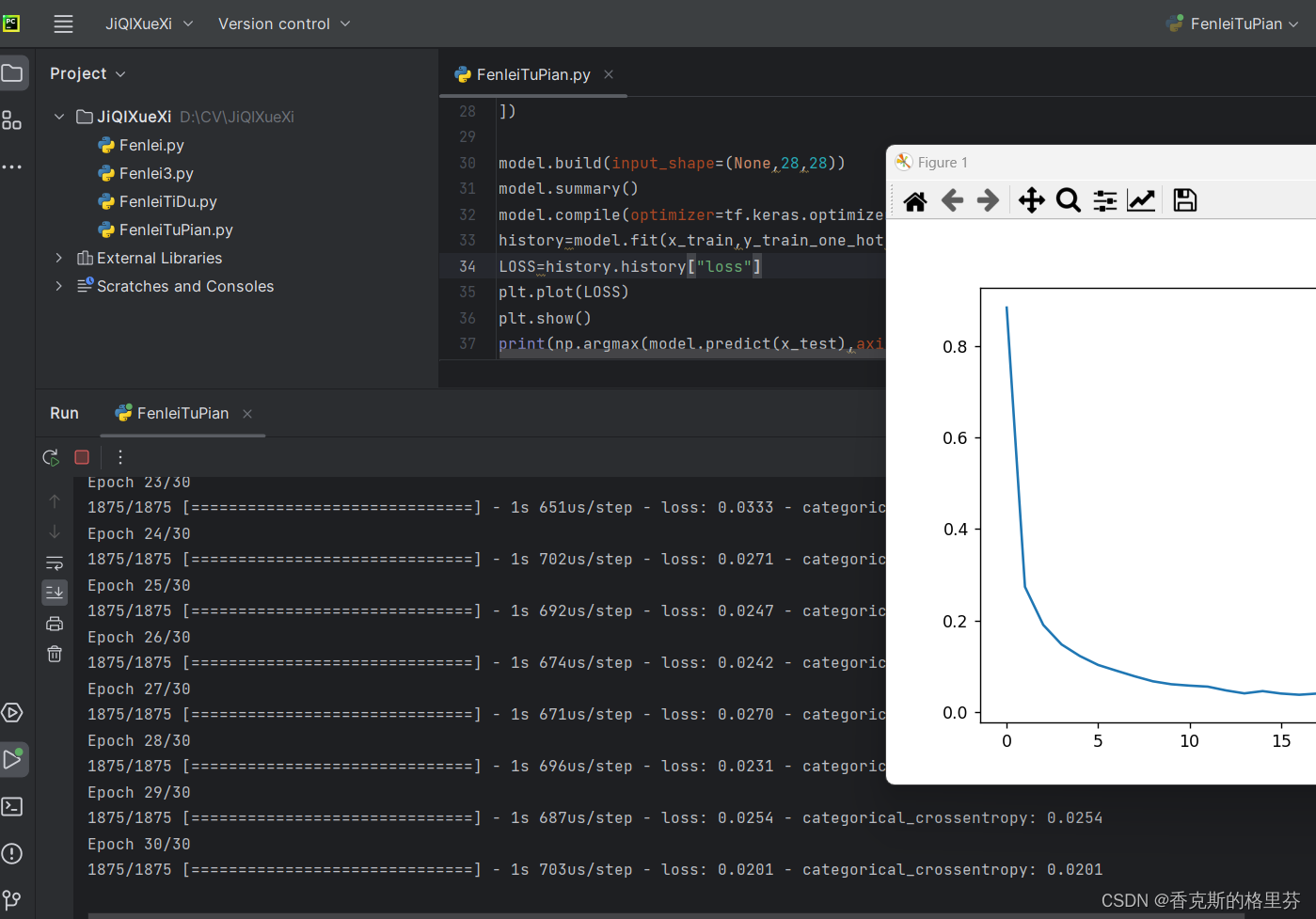
# 提取训练过程中的损失值  
LOSS = history.history["loss"]  
  
# 绘制损失值随epoch变化的曲线  
plt.plot(LOSS)  
plt.title('Training Loss')  
plt.xlabel('Epoch')  
plt.ylabel('Loss')  
plt.show()  
  
# 对测试集进行预测，并找到概率最大的类别（即预测的标签）  
# 注意：这里使用了np.argmax来获取最大值的索引，即预测的类别  
predictions = np.argmax(model.predict(x_test), axis=1)[:10]  
  
# 打印前10个测试样本的预测标签和真实标签  
print("Predicted labels:", predictions)  
print("True labels:", y_test[:10])

1. 数据加载：使用TensorFlow的内置数据集mnist加载手写数字图片和对应的标签。mnist数据集包含了60,000个训练样本和10,000个测试样本，每个样本都是一张28x28像素的灰度图片。

2. 数据预处理：将标签从整数形式转换为one-hot编码形式，以便模型进行多分类任务。例如，数字5将被转换为[0, 0, 0, 0, 0, 1, 0, 0, 0, 0]。

3. 模型构建：使用TensorFlow的Sequential API定义了一个简单的神经网络模型。这个模型由几个全连接层（Dense层）组成，每个层都使用了ReLU激活函数（除了输出层使用了softmax激活函数）。模型的输入是展平后的28x28像素图片，输出是10个类别的概率分布。

4. 模型编译：配置了模型的训练过程，包括优化器（这里使用了Adam优化器）、损失函数（这里使用了分类交叉熵损失函数CategoricalCrossentropy）和评估指标（这里使用了准确率Accuracy）。

5. 模型训练：使用训练数据对模型进行训练，通过调整模型的参数来最小化损失函数。这里训练了10个epoch。

6. 结果评估：使用测试数据对模型进行评估，计算了模型在测试集上的损失值，并绘制了损失随epoch变化的曲线。此外，还使用模型对测试集进行了预测，并打印了前10个样本的预测标签和真实标签，以便比较模型的性能。

2.从文件中寻找mnist.npz

可在网上自行下载。

import tensorflow as tf
import numpy as np
import matplotlib.pyplot as plt

# (x_train,y_train),(x_test,y_test)=tf.keras.datasets.mnist.load_data()
with np.load("mnist.npz") as f:
    x_train, y_train = f['x_train'], f['y_train']
    x_test, y_test = f['x_test'], f['y_test']
y_train_one_hot = tf.one_hot(y_train, 10).numpy()[:2000]
x_train = np.float32(x_train[:2000, :, :])
print(x_train.shape)
# print(y_train_one_hot[3])
# image=x_train[3]
# plt.imshow(image)
# plt.show()

model = tf.keras.Sequential([
    tf.keras.layers.Flatten(),
    tf.keras.layers.Dense(256, activation="relu"),
    tf.keras.layers.Dense(128, activation="relu"),
    tf.keras.layers.Dense(64, activation="relu"),
    tf.keras.layers.Dense(32, activation="relu"),
    tf.keras.layers.Dense(10, activation="softmax")
])

model.build(input_shape=[None, 28, 28])
model.summary()
model.compile(optimizer=tf.keras.optimizers.Adam(), loss=tf.keras.losses.CategoricalCrossentropy(),
              metrics=[tf.keras.losses.CategoricalCrossentropy()])
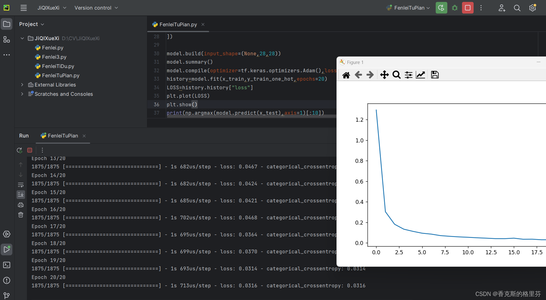
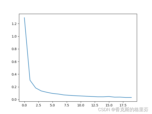
history = model.fit(x_train, y_train_one_hot, epochs=5)
LOSS = history.history["loss"]
plt.plot(LOSS)
plt.show()
print(np.argmax(model.predict(x_test), axis=1)[:10])
print(y_test[:10])

3.结果

epochs=10，损失函数降至0.0632

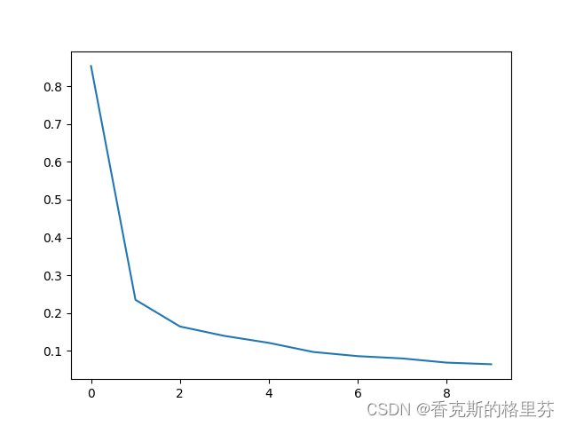
epochs=20，损失函数降至0.0336

epochs=30，损失函数降至0.0201

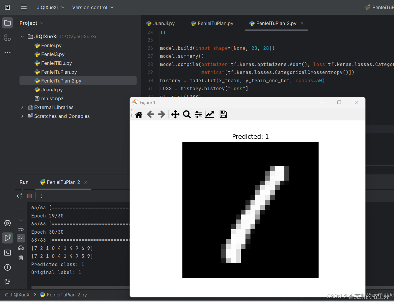
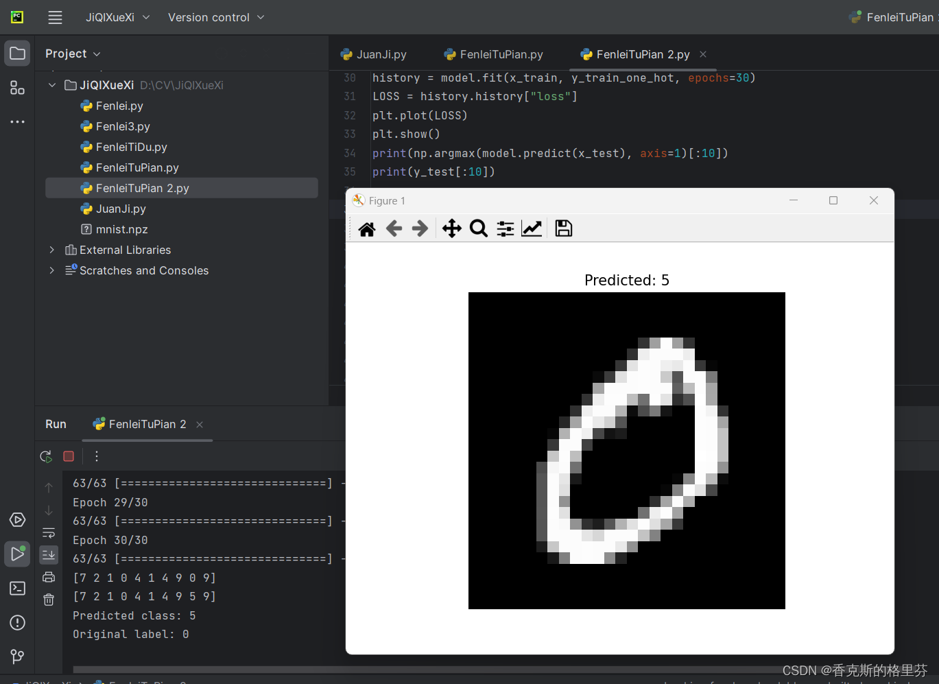
4.测试图片

# 假设我们想要测试训练集中的第3张图片
index = 3
test_image = x_train[index]  # 这里我们使用训练集的图片作为示例

# 归一化图片数据到0-1范围
test_image = test_image.astype('float32') / 255.0

# 扩展维度以适应模型的输入
test_image = np.expand_dims(test_image, axis=0)

# 使用模型进行预测
predictions = model.predict(test_image)

# 预测结果是一个概率分布，我们选择概率最高的类别
predicted_class = np.argmax(predictions)

# 输出预测结果和原始标签
print(f"Predicted class: {predicted_class}")
print(f"Original label: {y_train[index]}")

# 如果想要可视化预测的图片
plt.imshow(test_image[0], cmap='gray')
plt.title(f"Predicted: {predicted_class}")
plt.axis('off')
plt.show()

原始数据为1，预测数据为1

原始数据为0，预测数据为5