


因为之前一直用的Pytorch,这次是TensorFlow
●🍨 本文为🔗365天深度学习训练营 中的学习记录博客
●🍦 参考文章:365天深度学习训练营-第J1周:ResNet-50算法实战与解析
●🍖 原作者:K同学啊 | 接辅导、项目定制
目录
1.配置GPU ,没有这个就是默认CPU
具体来说,首先通过 tf.config.list_physical_devices("GPU") 获取当前可用的 GPU 设备列表,然后判断是否有可用的 GPU。如果有,则通过 tf.config.experimental.set_memory_growth(gpus[0], True) 设置第一块 GPU 按需使用显存,即显存会在需要时自动增加,而不是一开始就分配固定显存。接着,通过 tf.config.set_visible_devices([gpus[0],"GPU") 将第一块 GPU 设置为可见设备,即 TensorFlow 只会使用这一块 GPU。这样做可以保证 TensorFlow 在使用 GPU 时不会出现显存占用过高或者多个 CPU、GPU 设备之间的冲突等问题,从而获得更好的性能。
import tensorflow as tf

gpus = tf.config.list_physical_devices("GPU")

if gpus:
    tf.config.experimental.set_memory_growth(gpus[0], True)  #设置GPU显存用量按需使用
    tf.config.set_visible_devices([gpus[0]],"GPU")
2. 导入数据
import matplotlib.pyplot as plt
# 支持中文
plt.rcParams['font.sans-serif'] = ['SimHei']  # 用来正常显示中文标签
plt.rcParams['axes.unicode_minus'] = False  # 用来正常显示负号

import os,PIL,pathlib
import numpy as np

from tensorflow import keras
from tensorflow.keras import layers,models
data_dir = r"J1\bird_photos"
data_dir = pathlib.Path(data_dir)
3.查看
#查看数据
image_count = len(list(data_dir.glob('*/*')))

print("图片总数为:",image_count)
配置参数
batch_size = 8
img_height = 224
img_width = 224
二、数据预处理
这段代码使用 TensorFlow 中的 image_dataset_from_directory 函数从目录中加载图像数据集,并生成一个 tf.data.Dataset 对象,用于训练模型。
具体来说,代码中的 data_dir 变量表示图像数据集所在的文件夹路径,validation_split 表示将数据集分为训练集和验证集的比例,subset 表示当前生成的是训练集还是验证集(这里是训练集),seed 表示随机数种子,用于保证每次划分数据集时的结果一致。image_size 表示生成的图片大小,即将所有的图片转换为固定尺寸。batch_size 则表示每个 batch 包含的样本数量。
通过调用 image_dataset_from_directory 函数,可以快速创建一个数据集对象,并通过该对象获取到训练集的图片和标签数据,以便后续的训练过程。由于 tf.data.Dataset 对象可以自动进行数据的批处理、预处理等操作,因此使用该对象可以帮助我们更加高效地训练模型。
配置训练集
train_ds = tf.keras.preprocessing.image_dataset_from_directory(
    data_dir,
    validation_split=0.2,
    subset="training",
    seed=123,
    image_size=(img_height, img_width),
    batch_size=batch_size)
配置验证集
val_ds = tf.keras.preprocessing.image_dataset_from_directory(
    data_dir,
    validation_split=0.2,
    subset="validation",
    seed=123,
    image_size=(img_height, img_width),
    batch_size=batch_size)
查看类别
class_names = train_ds.class_names
print(class_names)#每个文件夹的名称就是对应的类别名称
2. 可视化数据
这段代码中的 plt.imshow(images[i].numpy().astype("uint8")) 用于显示一张图片。
具体来说,images 是一个形状为 (batch_size, image_height, image_width, channels) 的 Tensor 对象,其中 batch_size 是批次大小,image_height 和 image_width 分别是每张图片的高度和宽度,channels 是图片的通道数。在这里,我们通过 images[i] 获取到第 i 张图片,然后使用 numpy() 方法将其转换为 NumPy 数组类型,再使用 astype("uint8") 将像素值转换为 8 位整型(0~255),最后使用 plt.imshow 显示图片。
需要注意的是,plt.imshow 只能显示 RGB 三个通道的图片,如果图片的通道数不是 3,则需要进行转换或选择其中的某个通道来显示。此外,还可以通过 cmap 参数指定显示的颜色映射,以及通过 interpolation 参数指定插值方法来调整图片的显示效果。
plt.figure(figsize=(10, 5))  # 图形的宽为10高为5
plt.suptitle("查看数据")

for images, labels in train_ds.take(1):#train_ds.take(1) 从训练集中获取一个 batch 的图片和标签数据
    for i in range(8):

        ax = plt.subplot(2, 4, i + 1)

        plt.imshow(images[i].numpy().astype("uint8"))#astype("uint8") 将像素值转换为 8 位整型(0~255),最后使用 plt.imshow 显示图片。

        plt.title(class_names[labels[i]])

        plt.axis("off")#关闭坐标轴,以便更好地展示图片。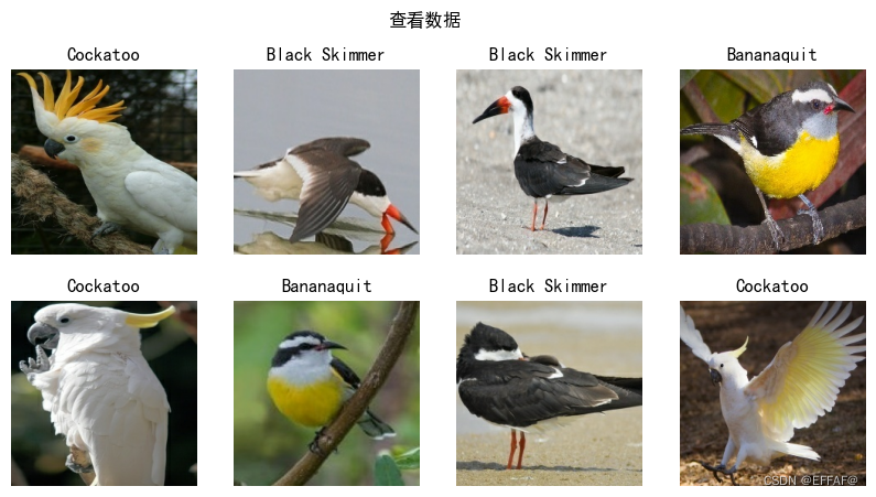
for image_batch, labels_batch in train_ds:
    print(image_batch.shape)
    print(labels_batch.shape)
    break
(8, 224, 224, 3) (8,)
4. 配置数据集
这段代码展示了如何使用 TensorFlow 的 tf.data 模块来构建可用于训练神经网络的数据集。其中 train_ds 和 val_ds 是对训练集和验证集的数据集对象的引用。这两个数据集都使用了缓存和预取机制来提高数据集的读取性能。
具体来说,cache() 方法通过缓存数据集到内存或磁盘中来避免重新读取数据,shuffle() 方法则对数据集进行洗牌,这样可以使得模型在训练时避免过拟合。
而 prefetch() 方法则允许模型在训练时并行地读取数据,从而加快了训练速度。其中 buffer_size 参数代表了要预取的数据的数量,在这里被设置为了 TensorFlow 自动调优的默认值 AUTOTUNE。这个值可以根据具体的运行环境和数据量进行调整,以达到最佳的性能表现。
AUTOTUNE = tf.data.AUTOTUNE
#tf.data 模块来构建可用于训练神经网络的数据集。其中 train_ds 和 val_ds 是对训练集和验证集的数据集对象的引用。
train_ds = train_ds.cache().shuffle(1000).prefetch(buffer_size=AUTOTUNE)
#cache() 方法通过缓存数据集到内存或磁盘中来避免重新读取数据,shuffle() 方法则对数据集进行洗牌,这样可以使得模型在训练时避免过拟合
# prefetch() 方法则允许模型在训练时并行地读取数据,从而加快了训练速度。其中 buffer_size 参数代表了要预取的数据的数量,在这里被设置为了 TensorFlow 自动调优的默认值 AUTOTUNE。
val_ds = val_ds.cache().prefetch(buffer_size=AUTOTUNE)
构建网络模型

from keras import layers

from keras.layers import Input,Activation,BatchNormalization,Flatten
from keras.layers import Dense,Conv2D,MaxPooling2D,ZeroPadding2D,AveragePooling2D
from keras.models import Model

def identity_block(input_tensor, kernel_size, filters, stage, block):

    filters1, filters2, filters3 = filters

    name_base = str(stage) + block + '_identity_block_'

    x = Conv2D(filters1, (1, 1), name=name_base + 'conv1')(input_tensor)
    x = BatchNormalization(name=name_base + 'bn1')(x)
    x = Activation('relu', name=name_base + 'relu1')(x)

    x = Conv2D(filters2, kernel_size,padding='same', name=name_base + 'conv2')(x)
    x = BatchNormalization(name=name_base + 'bn2')(x)
    x = Activation('relu', name=name_base + 'relu2')(x)

    x = Conv2D(filters3, (1, 1), name=name_base + 'conv3')(x)
    x = BatchNormalization(name=name_base + 'bn3')(x)

    x = layers.add([x, input_tensor] ,name=name_base + 'add')
    x = Activation('relu', name=name_base + 'relu4')(x)
    return x


def conv_block(input_tensor, kernel_size, filters, stage, block, strides=(2, 2)):

    filters1, filters2, filters3 = filters

    res_name_base = str(stage) + block + '_conv_block_res_'
    name_base = str(stage) + block + '_conv_block_'

    x = Conv2D(filters1, (1, 1), strides=strides, name=name_base + 'conv1')(input_tensor)
    x = BatchNormalization(name=name_base + 'bn1')(x)
    x = Activation('relu', name=name_base + 'relu1')(x)

    x = Conv2D(filters2, kernel_size, padding='same', name=name_base + 'conv2')(x)
    x = BatchNormalization(name=name_base + 'bn2')(x)
    x = Activation('relu', name=name_base + 'relu2')(x)

    x = Conv2D(filters3, (1, 1), name=name_base + 'conv3')(x)
    x = BatchNormalization(name=name_base + 'bn3')(x)

    shortcut = Conv2D(filters3, (1, 1), strides=strides, name=res_name_base + 'conv')(input_tensor)
    shortcut = BatchNormalization(name=res_name_base + 'bn')(shortcut)

    x = layers.add([x, shortcut], name=name_base+'add')
    x = Activation('relu', name=name_base+'relu4')(x)
    return x

def ResNet50(input_shape=[224,224,3],classes=1000):

    img_input = Input(shape=input_shape)
    x = ZeroPadding2D((3, 3))(img_input)

    x = Conv2D(64, (7, 7), strides=(2, 2), name='conv1')(x)
    x = BatchNormalization(name='bn_conv1')(x)
    x = Activation('relu')(x)
    x = MaxPooling2D((3, 3), strides=(2, 2))(x)

    x =     conv_block(x, 3, [64, 64, 256], stage=2, block='a', strides=(1, 1))
    x = identity_block(x, 3, [64, 64, 256], stage=2, block='b')
    x = identity_block(x, 3, [64, 64, 256], stage=2, block='c')

    x =     conv_block(x, 3, [128, 128, 512], stage=3, block='a')
    x = identity_block(x, 3, [128, 128, 512], stage=3, block='b')
    x = identity_block(x, 3, [128, 128, 512], stage=3, block='c')
    x = identity_block(x, 3, [128, 128, 512], stage=3, block='d')

    x =     conv_block(x, 3, [256, 256, 1024], stage=4, block='a')
    x = identity_block(x, 3, [256, 256, 1024], stage=4, block='b')
    x = identity_block(x, 3, [256, 256, 1024], stage=4, block='c')
    x = identity_block(x, 3, [256, 256, 1024], stage=4, block='d')
    x = identity_block(x, 3, [256, 256, 1024], stage=4, block='e')
    x = identity_block(x, 3, [256, 256, 1024], stage=4, block='f')

    x =     conv_block(x, 3, [512, 512, 2048], stage=5, block='a')
    x = identity_block(x, 3, [512, 512, 2048], stage=5, block='b')
    x = identity_block(x, 3, [512, 512, 2048], stage=5, block='c')

    x = AveragePooling2D((7, 7), name='avg_pool')(x)

    x = Flatten()(x)
    x = Dense(classes, activation='softmax', name='fc1000')(x)

    model = Model(img_input, x, name='resnet50')

    # 加载预训练模型
    model.load_weights(r"C:\Users\28625\Desktop\codeprogram\VC\pytorch\J1\resnet50_weights_tf_dim_ordering_tf_kernels.h5")

    return model

model = ResNet50()
model.summary()
编译
这段代码展示了如何使用 TensorFlow 的 Keras 模块来编译一个神经网络模型。其中,opt = tf.keras.optimizers.Adam(learning_rate=1e-7) 定义了一个优化器对象 opt,该优化器使用了 Adam 算法,并将学习率设置为 1e-7,即 0.0000001。
接着,使用 model.compile() 方法来编译模型。在这里,我们将损失函数(loss function)设为稀疏分类交叉熵(sparse_categorical_crossentropy),这个损失函数通常用于多分类问题中,其中目标类别是整数形式的。而 metrics 参数则定义了训练过程中要监测哪些指标(比如准确率、精确率等),这里我们监测了准确率(accuracy)。
需要注意的是,这里在编译模型时使用了 "adam" 作为 optimizer 参数,而并非前面定义的 opt 对象。这是因为在实际应用中,还可以通过其他方式来设置优化器,例如传递一个优化器名称或自定义的优化器对象,因此在这里我们采用这种更为通用的方式来编译模型。
# 设置优化器,我这里改变了学习率。
opt = tf.keras.optimizers.Adam(learning_rate=1e-7)

model.compile(optimizer="adam",
              loss='sparse_categorical_crossentropy',
              metrics=['accuracy'])
六、训练模型
这段代码展示了如何使用 TensorFlow 的 Keras 模块来训练一个神经网络模型。具体来说,model.fit() 方法用于拟合模型,并返回一个 History 对象,包含了训练过程中的一些重要信息。
在这里,train_ds 代表用于训练的数据集对象,validation_data 则代表用于验证的数据集对象。在训练时,模型将依次读取数据集中的每个批次(batch),并根据前面编译时指定的损失函数和优化器来更新模型的参数,从而逐渐减小损失值并提高分类准确率。
epochs 参数表示训练轮数,即遍历整个数据集的次数。在训练过程中,模型会多次读取数据集进行训练,每个轮数会使模型得到更好的学习。最终训练的结果将保存在 History 对象中,可以通过该对象的方法和属性来查看训练过程中的指标、损失值和准确率等信息
epochs = 10

history = model.fit(
    train_ds,
    validation_data=val_ds,
    epochs=epochs
)
查看数据
acc = history.history['accuracy']
val_acc = history.history['val_accuracy']

loss = history.history['loss']
val_loss = history.history['val_loss']

epochs_range = range(epochs)

plt.figure(figsize=(12, 4))
plt.subplot(1, 2, 1)
plt.suptitle("微信公众号:K同学啊")

plt.plot(epochs_range, acc, label='Training Accuracy')
plt.plot(epochs_range, val_acc, label='Validation Accuracy')
plt.legend(loc='lower right')
plt.title('Training and Validation Accuracy')

plt.subplot(1, 2, 2)
plt.plot(epochs_range, loss, label='Training Loss')
plt.plot(epochs_range, val_loss, label='Validation Loss')
plt.legend(loc='upper right')
plt.title('Training and Validation Loss')
plt.show()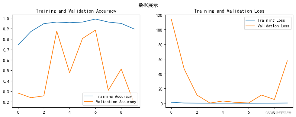
预测
# 采用加载的模型(new_model)来看预测结果

plt.figure(figsize=(10, 5))  # 图形的宽为10高为5
plt.suptitle("样例测试")

for images, labels in val_ds.take(1):
    for i in range(8):
        ax = plt.subplot(2, 4, i + 1)

        # 显示图片
        plt.imshow(images[i].numpy().astype("uint8"))

        # 需要给图片增加一个维度
        img_array = tf.expand_dims(images[i], 0)

        # 使用模型预测图片中的人物
        predictions = model.predict(img_array)
        plt.title(class_names[np.argmax(predictions)])

        plt.axis("off")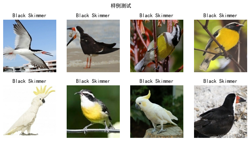


 1249
1249


 被折叠的 条评论
为什么被折叠?
被折叠的 条评论
为什么被折叠?
 到【灌水乐园】发言


