


🤵♂️ 个人主页:@艾派森的个人主页
✍🏻作者简介:Python学习者
🐋 希望大家多多支持,我们一起进步!😄
如果文章对你有帮助的话,
欢迎评论 💬点赞👍🏻 收藏 📂加关注+
目录
1.项目背景
在当今这个数据驱动的时代,数据分析与挖掘已成为企业决策的重要支撑。然而,随着数据量的爆炸性增长,如何高效、精准地进行数据分析与挖掘,成为了企业面临的重大挑战。幸运的是,随着人工智能技术的飞速发展,ChatGPT这一强大的自然语言处理模型,正逐渐成为数据分析与挖掘领域的新宠。
ChatGPT,全称为“Chat Generative Pre-trained Transformer”,是由美国人工智能公司OpenAI研发的一种基于深度学习技术的自然语言处理模型。它通过学习海量的文本数据,能够生成高质量、个性化的自然语言回应,实现了人机之间的无缝交互。ChatGPT的出现,不仅极大地推动了自然语言处理技术的发展,更为数据分析与挖掘领域带来了革命性的变化。
本次项目将聚焦于ChatGPT用户评论数据集的可视化分析。企业可以通过收集用户在电商平台上对商品的评论数据,利用ChatGPT强大的自然语言处理能力,对这些文本数据进行深度挖掘和可视化分析。通过这种方式,企业能够更直观地了解用户对不同产品的评价和反馈,进而优化产品设计和营销策略,提升用户满意度和转化率。
在具体实施中,企业可以将收集到的用户评论数据上传至ChatGPT系统,利用其自然语言处理能力对文本数据进行自动化处理与转化,将非结构化或半结构化的文本数据转化为结构化数据。随后,ChatGPT将对这些结构化数据进行深度分析,识别出用户对产品特征、购买意愿、满意度等方面的信息,并生成个性化的可视化图表,如柱状图、饼图、折线图等,展示销售额、用户数量、订单量等关键指标的变化趋势。这些图表不仅能够帮助决策者快速了解业务状况,还能够为企业的战略规划和决策制定提供有力支持。
此外,ChatGPT还能够根据用户的兴趣和偏好,生成个性化的商品推荐和营销策略,提高用户满意度和转化率。同时,它还可以根据用户的反馈和行为数据,不断优化推荐算法和营销策略,提升用户体验和企业的市场竞争力。
综上所述,通过利用ChatGPT对用户评论数据集进行可视化分析,企业能够更深入地了解用户需求和市场趋势,为产品优化和营销策略制定提供有力支持,进而在激烈的市场竞争中立于不败之地,实现可持续发展。
2.数据集介绍
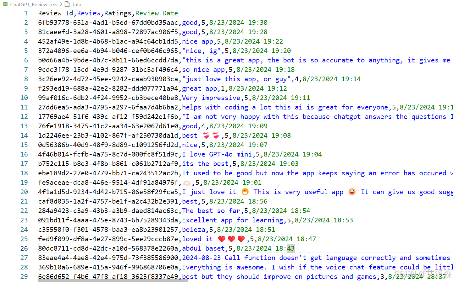
本数据集来源于Kaggle,该数据集由ChatGPT的用户评论组成,包括文本反馈、评分和评论日期。评论范围从简短评论到更详细的反馈,涵盖了广泛的用户情绪。评分范围从 1 到 5,代表不同的满意度水平。数据集跨越多个月,为分析提供了时间维度。每条评论都附有时间戳,可以对情绪趋势进行时间序列分析。
3.技术工具
Python版本:3.9
代码编辑器:jupyter notebook
4.导入数据
导入第三方库并加载数据集
import numpy as np
import pandas as pd
from wordcloud import WordCloud
from textblob import TextBlob
import matplotlib.pyplot as plt
from collections import Counter
from nltk.corpus import stopwords
import string

df = pd.read_csv('ChatGPT_Reviews.csv')
df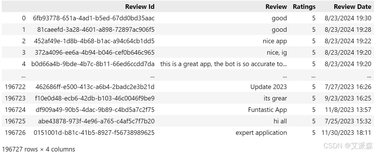
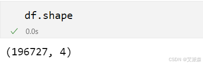
查看数据大小
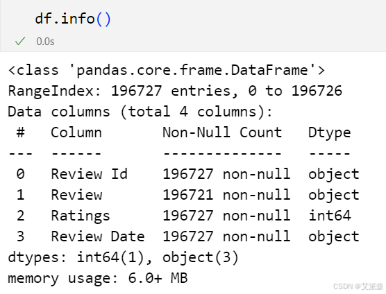
查看数据基本信息
对评论日期和评分变量进行处理
# 将评论日期转为日期类型,无法转换的异常数据设置为空值
df['Review Date'] = pd.to_datetime(df['Review Date'], errors='coerce')
# 将评分转为数值类型,无法转换的异常数据设置为空值
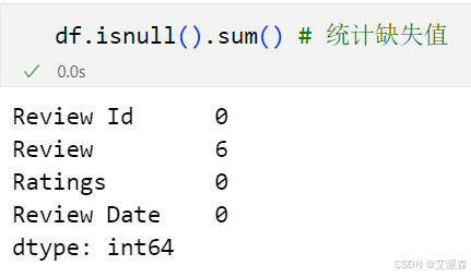
df['Ratings'] = pd.to_numeric(df['Ratings'], errors='coerce') 统计缺失值
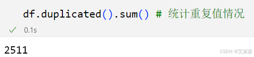
统计重复值
5.数据可视化

# 评分分布
def plot_ratings_distribution(df):
    plt.hist(df['Ratings'], bins=5, edgecolor='black', color='skyblue')
    plt.title("Ratings Distribution")
    plt.xlabel("Ratings")
    plt.ylabel("Frequency")
    plt.show()

plot_ratings_distribution(df)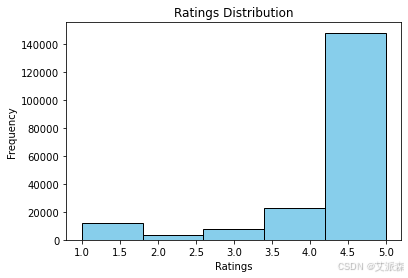
# 对评论进行情感分析
def analyze_sentiments(df):
    def analyze_sentiment(text):
        analysis = TextBlob(text)
        return analysis.polarity

    df['Sentiment'] = df['Review'].apply(analyze_sentiment)
    plt.hist(df['Sentiment'], bins=20, color='lightgreen', edgecolor='black')
    plt.title("Sentiment Polarity Distribution")
    plt.xlabel("Polarity")
    plt.ylabel("Frequency")
    plt.show()
    return df

analyze_sentiments(df)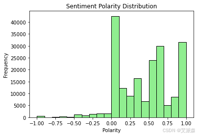
# 情绪极性与评级的散点图
def plot_sentiment_vs_ratings(df):
    plt.scatter(df['Sentiment'], df['Ratings'], alpha=0.5, color='purple')
    plt.title("Sentiment Polarity vs Ratings")
    plt.xlabel("Sentiment Polarity")
    plt.ylabel("Ratings")
    plt.show()

plot_sentiment_vs_ratings(df)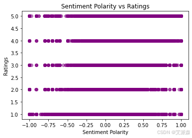
# 生成并显示评论的词云
def generate_word_cloud(df):
    text = " ".join(review for review in df['Review'])
    wordcloud = WordCloud(width=800, height=400, background_color='white').generate(text)
    plt.figure(figsize=(10, 5))
    plt.imshow(wordcloud, interpolation='bilinear')
    plt.axis("off")
    plt.show()

generate_word_cloud(df)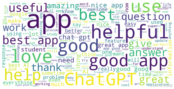
# 分析评级和情绪的时间趋势
def temporal_trends(df):
    df['Review Month'] = df['Review Date'].dt.to_period('M')
    monthly_avg_ratings = df.groupby('Review Month')['Ratings'].mean()
    monthly_avg_sentiment = df.groupby('Review Month')['Sentiment'].mean()

    months = monthly_avg_ratings.index.astype(str)

    plt.figure(figsize=(12, 6))
    plt.plot(months, monthly_avg_ratings, label='Average Ratings', marker='o', color='blue')
    plt.plot(months, monthly_avg_sentiment, label='Average Sentiment', marker='o', color='green')
    plt.title("Temporal Trends: Ratings and Sentiments")
    plt.xlabel("Month")
    plt.ylabel("Average Value")
    plt.legend()
    plt.grid()
    plt.xticks(rotation=45)
    plt.tight_layout()
    plt.show()

temporal_trends(df)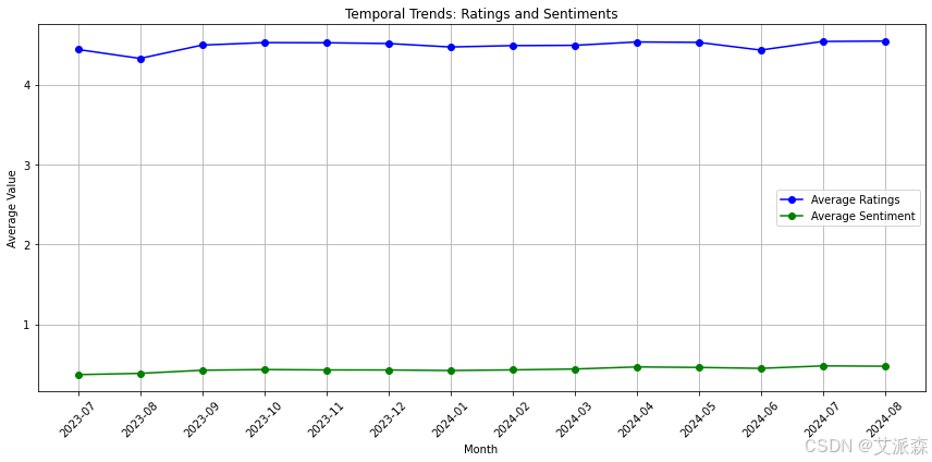
确定每个评级类别(例如,1星,5星)评论中使用频率最高的单词。
def get_top_words(reviews, n=10):
    stop_words = set(stopwords.words('english'))
    words = " ".join(reviews).lower().translate(str.maketrans('', '', string.punctuation)).split()
    words = [word for word in words if word not in stop_words]
    return Counter(words).most_common(n)

for rating in df['Ratings'].unique():
    top_words = get_top_words(df[df['Ratings'] == rating]['Review'], n=10)
    print(f"Top words for rating {rating}: {top_words}")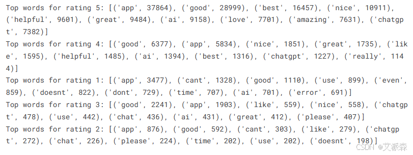
# 临时评论计数趋势分析一段时间内提交的评论数量,以确定高用户活动的时期
review_counts = df.groupby(df['Review Date'].dt.to_period('M')).size()
review_counts.plot(kind='bar', color='skyblue', figsize=(12, 6))
plt.title("Number of Reviews Over Time")
plt.xlabel("Month")
plt.ylabel("Number of Reviews")
plt.xticks(rotation=45)
plt.tight_layout()
plt.show()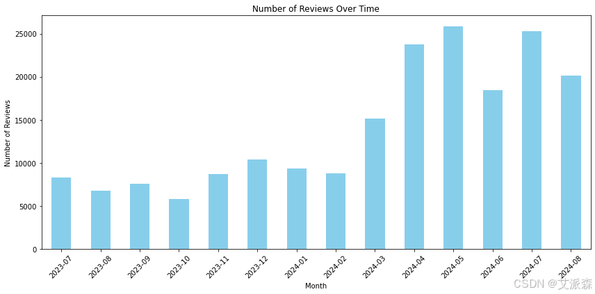
import seaborn as sns
def categorize_sentiment(polarity):
    if polarity > 0.2:
        return "Positive"
    elif polarity < -0.2:
        return "Negative"
    else:
        return "Neutral"

if 'Sentiment' in df.columns:
    df['Sentiment Category'] = df['Sentiment'].apply(categorize_sentiment)
else:
    print("Error: 'Sentiment' column not found. Ensure sentiment analysis has been performed.")

print(df.columns)
heatmap_data = df.pivot_table(index='Ratings', columns='Sentiment Category', aggfunc='size', fill_value=0)
sns.heatmap(heatmap_data, annot=True, fmt='d', cmap='coolwarm')
plt.title("Ratings vs Sentiment Categories")
plt.xlabel("Sentiment Category")
plt.ylabel("Ratings")
plt.show() 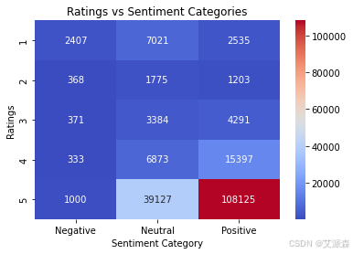
# 不同时期的情感变化趋势
sentiment_trend = df.groupby([df['Review Date'].dt.to_period('M'), 'Sentiment Category']).size().unstack(fill_value=0)
sentiment_trend.plot(kind='area', stacked=True, figsize=(12, 6), colormap='coolwarm')
plt.title("Sentiment Distribution Over Time")
plt.xlabel("Month")
plt.ylabel("Number of Reviews")
plt.legend(title="Sentiment Category")
plt.xticks(rotation=45)
plt.tight_layout()
plt.show()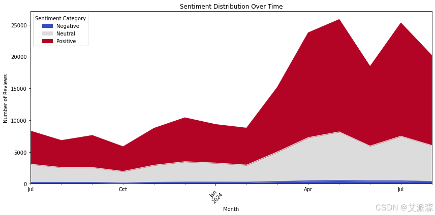
# 分析不同长度评论的情感
df['Review Length'] = df['Review'].str.len()
df['Length Category'] = pd.cut(df['Review Length'],
                               bins=[0, 50, 150, 300, 1000],
                               labels=['Short', 'Medium', 'Long', 'Very Long'])
length_sentiment = pd.crosstab(df['Length Category'], df['Sentiment Category'])
length_sentiment.plot(kind='bar', stacked=True, figsize=(12, 6), colormap='viridis')
plt.title("Review Length vs Sentiment Category")
plt.xlabel("Length Category")
plt.ylabel("Number of Reviews")
plt.legend(title="Sentiment Category")
plt.show()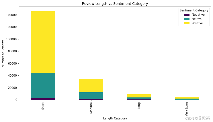
文末推荐
《巧用DeepSeek快速搞定数据分析》

内容简介
本书是一本关于数据分析与DeepSeek应用的实用指南,旨在帮助读者了解数据分析的基础知识及如何利用DeepSeek进行高效的数据处理和分析。随着大数据时代的到来,数据分析已经成为现代企业和行业发展的关键驱动力,本书正是为了满足这一市场需求而诞生。
本书共分为8章,涵盖了从数据分析基础知识、常见的统计学方法,到使用DeepSeek进行数据准备、数据清洗、特征提取、数据可视化、回归分析与预测建模、分类与聚类分析及深度学习和大数据分析等全面的内容。各章节详细介绍了如何运用DeepSeek在数据分析过程中解决实际问题,并提供了丰富的实例以帮助读者快速掌握相关技能。
本书适合数据分析师、数据科学家、研究人员、企业管理者、学生及对数据分析和人工智能技术感兴趣的广大读者阅读。通过阅读本书,读者将掌握数据分析的核心概念和方法,并学会如何运用DeepSeek为数据分析工作带来更高的效率和价值。
源代码
import numpy as np
import pandas as pd
from wordcloud import WordCloud
from textblob import TextBlob
import matplotlib.pyplot as plt
from collections import Counter
from nltk.corpus import stopwords
import string

df = pd.read_csv('ChatGPT_Reviews.csv')
df
df.shape
df.info()
# 将评论日期转为日期类型,无法转换的异常数据设置为空值
df['Review Date'] = pd.to_datetime(df['Review Date'], errors='coerce')
# 将评分转为数值类型,无法转换的异常数据设置为空值
df['Ratings'] = pd.to_numeric(df['Ratings'], errors='coerce')
df.isnull().sum() # 统计缺失值
df.dropna(inplace=True) # 删除缺失值
df.duplicated().sum() # 统计重复值情况
df.drop_duplicates(inplace=True) # 删除重复值
# 评分分布
def plot_ratings_distribution(df):
    plt.hist(df['Ratings'], bins=5, edgecolor='black', color='skyblue')
    plt.title("Ratings Distribution")
    plt.xlabel("Ratings")
    plt.ylabel("Frequency")
    plt.show()

plot_ratings_distribution(df)
# 对评论进行情感分析
def analyze_sentiments(df):
    def analyze_sentiment(text):
        analysis = TextBlob(text)
        return analysis.polarity

    df['Sentiment'] = df['Review'].apply(analyze_sentiment)
    plt.hist(df['Sentiment'], bins=20, color='lightgreen', edgecolor='black')
    plt.title("Sentiment Polarity Distribution")
    plt.xlabel("Polarity")
    plt.ylabel("Frequency")
    plt.show()
    return df

analyze_sentiments(df)
# 情绪极性与评级的散点图
def plot_sentiment_vs_ratings(df):
    plt.scatter(df['Sentiment'], df['Ratings'], alpha=0.5, color='purple')
    plt.title("Sentiment Polarity vs Ratings")
    plt.xlabel("Sentiment Polarity")
    plt.ylabel("Ratings")
    plt.show()

plot_sentiment_vs_ratings(df)
# 生成并显示评论的词云
def generate_word_cloud(df):
    text = " ".join(review for review in df['Review'])
    wordcloud = WordCloud(width=800, height=400, background_color='white').generate(text)
    plt.figure(figsize=(10, 5))
    plt.imshow(wordcloud, interpolation='bilinear')
    plt.axis("off")
    plt.show()

generate_word_cloud(df)
# 分析评级和情绪的时间趋势
def temporal_trends(df):
    df['Review Month'] = df['Review Date'].dt.to_period('M')
    monthly_avg_ratings = df.groupby('Review Month')['Ratings'].mean()
    monthly_avg_sentiment = df.groupby('Review Month')['Sentiment'].mean()

    months = monthly_avg_ratings.index.astype(str)

    plt.figure(figsize=(12, 6))
    plt.plot(months, monthly_avg_ratings, label='Average Ratings', marker='o', color='blue')
    plt.plot(months, monthly_avg_sentiment, label='Average Sentiment', marker='o', color='green')
    plt.title("Temporal Trends: Ratings and Sentiments")
    plt.xlabel("Month")
    plt.ylabel("Average Value")
    plt.legend()
    plt.grid()
    plt.xticks(rotation=45)
    plt.tight_layout()
    plt.show()

temporal_trends(df)
def get_top_words(reviews, n=10):
    stop_words = set(stopwords.words('english'))
    words = " ".join(reviews).lower().translate(str.maketrans('', '', string.punctuation)).split()
    words = [word for word in words if word not in stop_words]
    return Counter(words).most_common(n)

for rating in df['Ratings'].unique():
    top_words = get_top_words(df[df['Ratings'] == rating]['Review'], n=10)
    print(f"Top words for rating {rating}: {top_words}")
# 临时评论计数趋势分析一段时间内提交的评论数量,以确定高用户活动的时期
review_counts = df.groupby(df['Review Date'].dt.to_period('M')).size()
review_counts.plot(kind='bar', color='skyblue', figsize=(12, 6))
plt.title("Number of Reviews Over Time")
plt.xlabel("Month")
plt.ylabel("Number of Reviews")
plt.xticks(rotation=45)
plt.tight_layout()
plt.show()
import seaborn as sns
def categorize_sentiment(polarity):
    if polarity > 0.2:
        return "Positive"
    elif polarity < -0.2:
        return "Negative"
    else:
        return "Neutral"

if 'Sentiment' in df.columns:
    df['Sentiment Category'] = df['Sentiment'].apply(categorize_sentiment)
else:
    print("Error: 'Sentiment' column not found. Ensure sentiment analysis has been performed.")

print(df.columns)
heatmap_data = df.pivot_table(index='Ratings', columns='Sentiment Category', aggfunc='size', fill_value=0)
sns.heatmap(heatmap_data, annot=True, fmt='d', cmap='coolwarm')
plt.title("Ratings vs Sentiment Categories")
plt.xlabel("Sentiment Category")
plt.ylabel("Ratings")
plt.show()
# 不同时期的情感变化趋势
sentiment_trend = df.groupby([df['Review Date'].dt.to_period('M'), 'Sentiment Category']).size().unstack(fill_value=0)
sentiment_trend.plot(kind='area', stacked=True, figsize=(12, 6), colormap='coolwarm')
plt.title("Sentiment Distribution Over Time")
plt.xlabel("Month")
plt.ylabel("Number of Reviews")
plt.legend(title="Sentiment Category")
plt.xticks(rotation=45)
plt.tight_layout()
plt.show()
# 分析不同长度评论的情感
df['Review Length'] = df['Review'].str.len()
df['Length Category'] = pd.cut(df['Review Length'],
                               bins=[0, 50, 150, 300, 1000],
                               labels=['Short', 'Medium', 'Long', 'Very Long'])
length_sentiment = pd.crosstab(df['Length Category'], df['Sentiment Category'])
length_sentiment.plot(kind='bar', stacked=True, figsize=(12, 6), colormap='viridis')
plt.title("Review Length vs Sentiment Category")
plt.xlabel("Length Category")
plt.ylabel("Number of Reviews")
plt.legend(title="Sentiment Category")
plt.show()
资料获取,更多粉丝福利,关注下方公众号获取


 2万+
2万+

 被折叠的 条评论
为什么被折叠?
被折叠的 条评论
为什么被折叠?
 到【灌水乐园】发言


