数据挖掘实战-基于随机森林算法的交通事故预测模型

最新推荐文章于 2025-04-28 23:46:40 发布

置顶艾派森

最新推荐文章于 2025-04-28 23:46:40 发布

阅读量7.9k

点赞数 41

分类专栏： Pyhton数据分析文章标签：数据挖掘算法随机森林人工智能信息可视化

本文链接：https://blog.csdn.net/m0_64336780/article/details/145355381

版权

Pyhton数据分析专栏收录该内容

21 篇文章

订阅专栏

🤵‍♂️ 个人主页：@艾派森的个人主页

✍🏻作者简介：Python学习者
🐋 希望大家多多支持，我们一起进步！😄
如果文章对你有帮助的话，
欢迎评论 💬点赞👍🏻 收藏 📂加关注+

1.项目背景

随着车辆数量的不断增加和交通网络的日益扩大，交通事故的风险也在持续上升。这些事故不仅给人们的日常生活带来了诸多不便，还对社会经济造成了巨大的影响。为了有效应对这一问题，建立一种高效的交通事故预测模型显得尤为重要。这种模型能够帮助我们更好地预测和防范交通事故，从而提高道路交通安全水平，并减少由此带来的社会经济损失。

交通事故的发生往往受到多种因素的影响，包括驾驶员的人为因素（如超速、疲劳驾驶、酒驾等）以及自然因素（如天气、道路环境等）。通过对历史交通事故数据的深入分析，我们可以揭示出事故发生的规律和主要风险因素，从而为预测和防范交通事故提供有力的支持。而数据挖掘技术，特别是机器学习算法，在这方面展现出了巨大的潜力。

随机森林算法作为一种非常成功的集成学习算法，在分类和回归等多个领域都展现出了卓越的性能。它通过构建多个决策树，并对这些树的预测结果进行综合，从而形成一个强大的预测模型。与单一决策树相比，随机森林具有显著降低过拟合风险和提高预测准确性的优势。因此，将随机森林算法应用于交通事故预测模型，有望提高模型的预测性能和准确性。

在实际应用中，我们可以利用历史交通事故数据来训练随机森林模型。通过对数据的处理和特征的筛选，我们可以得到更加准确的交通事故预测结果。这些预测结果可以应用于城市交通管理、交通规划和交通安全管理等多个领域。例如，在交通规划方面，我们可以根据对未来交通事故的预测结果进行道路建设规划和布局；在交通安全管理方面，我们可以通过早期预测交通事故风险，及时采取措施进行预防和救援，从而减少交通事故对人民群众的影响。

此外，值得注意的是，虽然随机森林算法在交通事故预测中表现出了较高的准确性，但仍存在一些改进空间。例如，随机森林构建的是一种黑箱模型，其可解释性相对较弱。因此，在未来的研究中，我们可以尝试将随机森林与其他模型结合组成新的模型来分析交通事故，以提高其准确率和可解释性。同时，在数据记录和搜集方面，我们也可以更加细致地划分特征变量的属性等级，以更好地反映某些特征的重要性。

综上所述，基于随机森林算法的交通事故预测模型在数据挖掘实战中具有重要的研究价值和应用前景。它能够帮助我们更好地预测和防范交通事故，提高道路交通安全水平，并为社会经济发展提供有力保障。

2.数据集介绍

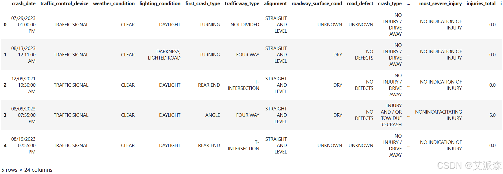
本实验数据集来源于Kaggle，原始数据集共有209306条，该数据集包含不同地区和时间段的交通事故详细信息。它包括各种指标，例如事故日期、天气状况、照明条件、碰撞类型、受伤人数和车辆参与情况。数据涵盖多个地点和事故类型，可全面了解交通事故及其原因。具体包括：

crash_date：事故发生的日期。

Traffic_control_device：所涉及的交通控制设备的类型（例如交通灯、标志）。

weather_condition：事故发生时的天气状况。

lighting_condition：事故发生时的照明条件。

first_crash_type：碰撞的初始类型（例如，迎面碰撞、追尾碰撞）。

Trafficway_type：发生事故的道路类型（例如高速公路、地方道路）。

路线：发生事故的道路的路线（例如直线、曲线）。

roadway_surface_cond：道路表面状况（例如干燥、潮湿、结冰）。

road_defect：道路表面上存在的任何缺陷。

crash_type：崩溃的总体类型。

cross_related_i：事故是否与交叉路口有关。

损害：事故造成的损害程度。

prim_contributory_cause：导致崩溃的主要原因。

num_units：涉及事故的车辆数量。

most_severe_injury：事故中遭受的最严重的伤害。

injury_total：报告的受伤总数。

injury_fatal：事故造成的致命伤害人数。

injury_incapacitating：致残伤害的数量。

injury_non_incapacitating：非致残性伤害的数量。

injury_reported_not_evident：已报告但并不明显的受伤人数。

injury_no_indication：没有受伤迹象的病例数。

crash_hour：事故发生的时间。

crash_day_of_week：事故发生的星期几。

crash_month：事故发生的月份。

用例：

事故分析：分析不同地点、时间段和条件下的事故趋势、类型和伤害严重程度。

交通安全：了解导致事故的因素（例如天气、灯光、道路状况），以便采取交通安全措施。

预测模型：使用数据集预测事故热点、潜在伤害以及各种因素对事故严重程度的影响。

3.技术工具

Python版本:3.9

代码编辑器：jupyter notebook

4.实验过程

4.1导入数据

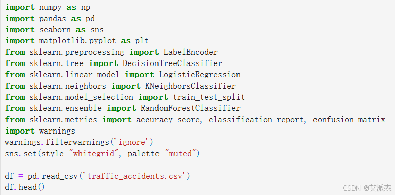
导入第三方库并加载数据集

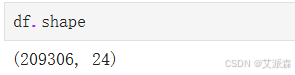
查看数据大小

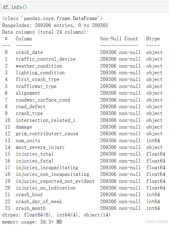
查看数据基本信息

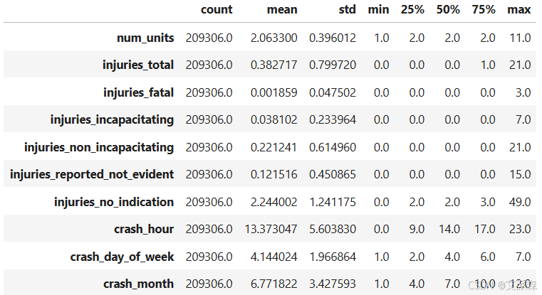
查看数值型变量的描述性统计

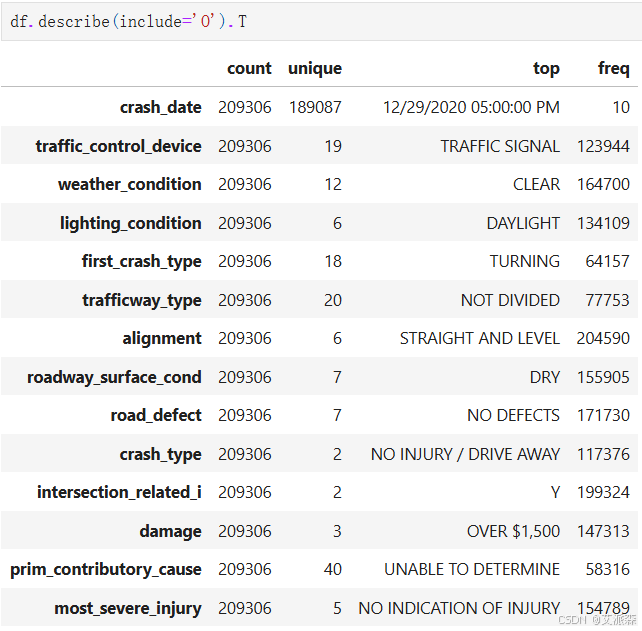
查看非数值型变量的描述性统计

4.2数据预处理

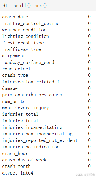
统计缺失值情况

统计重复值情况

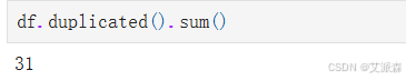
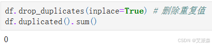
发现存在重复值，删除即可

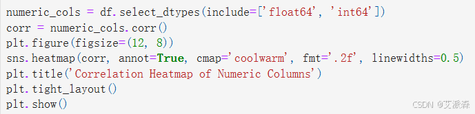
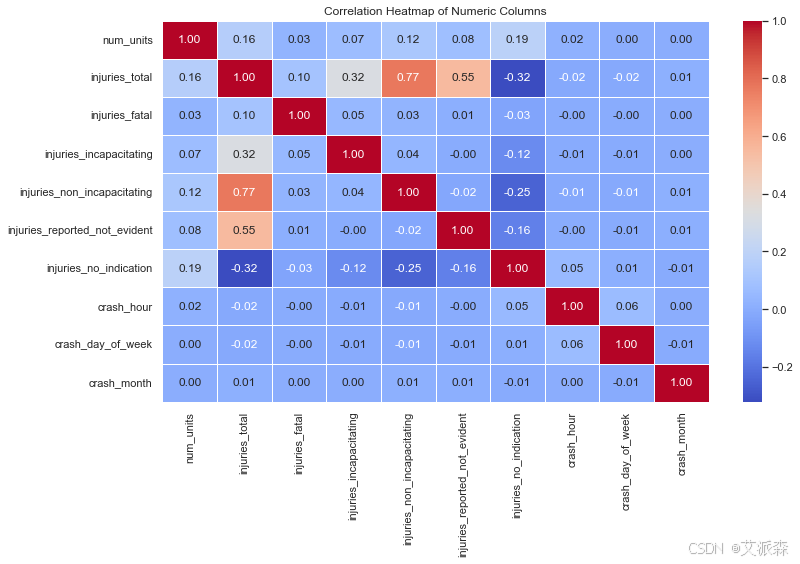
4.3数据可视化

4.4特征工程

编码处理

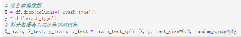
准备建模数据，并拆分数据集

4.5构建模型

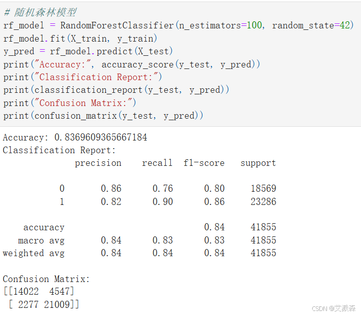
4.6模型评估

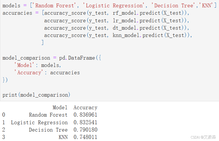
从构建的四个模型中，可以看出随机森林模型准确度最高，故选其作为最终模型。

特征重要性

# 特征重要性
Feature_importances = rf_model.feature_importances_
sorted_indices = np.argsort(Feature_importances)

plt.figure(figsize=(10, 5))
plt.barh(np.array(X.columns)[sorted_indices], Feature_importances[sorted_indices], color=plt.cm.rainbow(np.linspace(0, 1, len(Feature_importances))), alpha=0.7)
plt.title("Feature Importances - Random Forest")
plt.xlabel("Importance")
plt.tight_layout()
plt.show()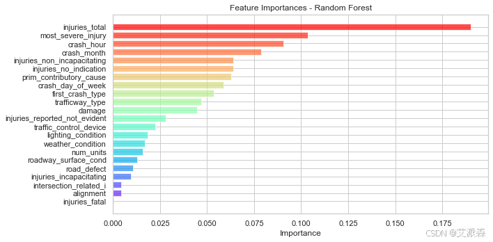

文末推荐

《Python区块链应用开发从入门到精通》

内容简介

本书全面系统地介绍了Python语言区块链应用工程师所需的基础知识和相关技术，主要分为Python基础篇、区块链技术篇和区块链开发篇三部分。

全书共10章，其中第1~3章为Python基础篇，介绍Python语法基础、Python的语法特色、Python与数据库操作等内容；第4~6章为区块链技术篇，介绍初始区块链、区块链的技术原理、区块链技术的发展趋势；第7~10章为区块链开发篇，介绍Solidity智能合约开发的入门和进阶、Python语言离线钱包开发、通过Python和Solidity开发一个“悬赏任务系统”，项目中将使用FISCO BCOS联盟链作为基础，结合Django框架，并应用Python-SDK与区块链交互完成数据的读写操作，完成一个区块链的Web项目。

本书内容系统全面，案例丰富详实，既适合想学习Python语言编程和区块链开发的初学者阅读，也适合作为区块链行业从业者、金融科技爱好者的学习用书，还可以作为广大职业院校相关专业的教材参考用书。

京东购买链接：https://item.jd.com/14356123.html

当当购买链接：https://product.dangdang.com/29827519.html

《AI智能化办公：讯飞星火AI使用方法与技巧从入门到精通》

内容简介

本书以讯飞星火认知大模型为例，全面系统地阐述其基础知识、操作方法与技巧，以及相关实战案例。全书共分为12章，第1章为新手入门篇，为读者铺垫了讯飞星火认知大模型（以下简称讯飞星火）的基础知识；第2至第4章为基础操作篇，提供了讯飞星火的基础操作、对讯飞星火插件的探索以及讯飞星火指令集的详解；第5至第10章为应用实战篇，深入剖析了讯飞星火在办公自动化、编程辅助、创意绘画、专业设计、艺术摄影等多个维度的深度应用，并结合实际案例进行阐释；第11章～第12章为进阶拓展篇，一方面介绍了更多整合讯飞星火技术的AI产品，另一方面着眼于讯飞星火与信息检索技术结合的前沿创新。

本书采用通俗易懂的语言和紧贴现实需求的案例，旨在为广大对人工智能兴趣浓厚的读者群体提供一本实用指南。无论您是刚踏入AI领域的新手，还是有着丰富经验的资深专业人士，阅读本书都将助您拓宽知识视野，激发创造灵感。

京东购买链接：https://item.jd.com/14349955.html

当当购买链接：https://product.dangdang.com/29821292.html

源代码

该数据集包含不同地区和时间段的交通事故详细信息。它包括各种指标，例如事故日期、天气状况、照明条件、碰撞类型、受伤人数和车辆参与情况。数据涵盖多个地点和事故类型，可全面了解交通事故及其原因。


crash_date：事故发生的日期。
Traffic_control_device：所涉及的交通控制设备的类型（例如交通灯、标志）。
weather_condition：事故发生时的天气状况。
lighting_condition：事故发生时的照明条件。
first_crash_type：碰撞的初始类型（例如，迎面碰撞、追尾碰撞）。
Trafficway_type：发生事故的道路类型（例如高速公路、地方道路）。
路线：发生事故的道路的路线（例如直线、曲线）。
roadway_surface_cond：道路表面状况（例如干燥、潮湿、结冰）。
road_defect：道路表面上存在的任何缺陷。
crash_type：崩溃的总体类型。
cross_related_i：事故是否与交叉路口有关。
损害：事故造成的损害程度。
prim_contributory_cause：导致崩溃的主要原因。
num_units：涉及事故的车辆数量。
most_severe_injury：事故中遭受的最严重的伤害。
injury_total：报告的受伤总数。
injury_fatal：事故造成的致命伤害人数。
injury_incapacitating：致残伤害的数量。
injury_non_incapacitating：非致残性伤害的数量。
injury_reported_not_evident：已报告但并不明显的受伤人数。
injury_no_indication：没有受伤迹象的病例数。
crash_hour：事故发生的时间。
crash_day_of_week：事故发生的星期几。
crash_month：事故发生的月份。
用例：
事故分析：分析不同地点、时间段和条件下的事故趋势、类型和伤害严重程度。
交通安全：了解导致事故的因素（例如天气、灯光、道路状况），以便采取交通安全措施。
预测模型：使用数据集预测事故热点、潜在伤害以及各种因素对事故严重程度的影响。
import numpy as np
import pandas as pd
import seaborn as sns
import matplotlib.pyplot as plt
from sklearn.preprocessing import LabelEncoder
from sklearn.tree import DecisionTreeClassifier
from sklearn.linear_model import LogisticRegression
from sklearn.neighbors import KNeighborsClassifier
from sklearn.model_selection import train_test_split
from sklearn.ensemble import RandomForestClassifier
from sklearn.metrics import accuracy_score, classification_report, confusion_matrix
import warnings
warnings.filterwarnings('ignore')
sns.set(style="whitegrid", palette="muted")

df = pd.read_csv('traffic_accidents.csv')
df.head()
df.shape
df.info()
df.describe().T
df.describe(include='O').T
df.isnull().sum()
df.duplicated().sum()
df.drop_duplicates(inplace=True) # 删除重复值
df.duplicated().sum()
numeric_cols = df.select_dtypes(include=['float64', 'int64'])
corr = numeric_cols.corr()
plt.figure(figsize=(12, 8))
sns.heatmap(corr, annot=True, cmap='coolwarm', fmt='.2f', linewidths=0.5)
plt.title('Correlation Heatmap of Numeric Columns')
plt.tight_layout()
plt.show()
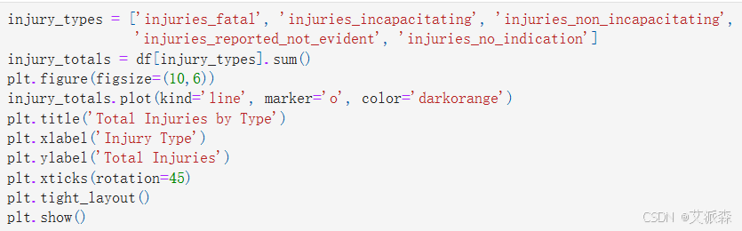
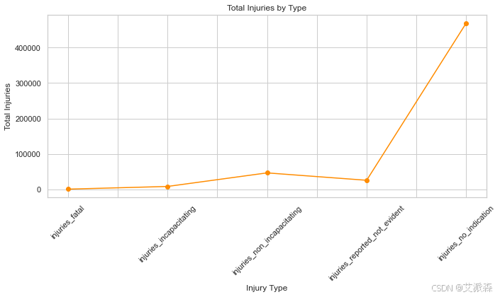
injury_types = ['injuries_fatal', 'injuries_incapacitating', 'injuries_non_incapacitating', 
                'injuries_reported_not_evident', 'injuries_no_indication']
injury_totals = df[injury_types].sum()
plt.figure(figsize=(10,6))
injury_totals.plot(kind='line', marker='o', color='darkorange')
plt.title('Total Injuries by Type')
plt.xlabel('Injury Type')
plt.ylabel('Total Injuries')
plt.xticks(rotation=45)
plt.tight_layout()
plt.show()

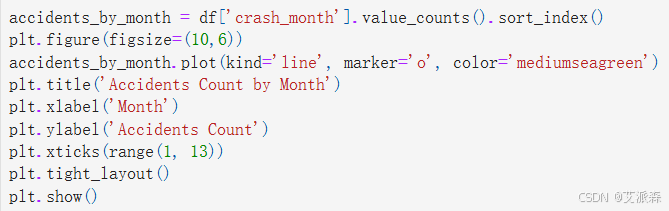
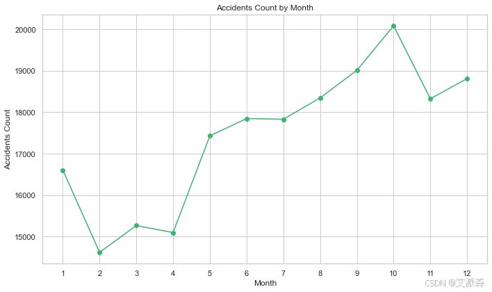
accidents_by_month = df['crash_month'].value_counts().sort_index()
plt.figure(figsize=(10,6))
accidents_by_month.plot(kind='line', marker='o', color='mediumseagreen')
plt.title('Accidents Count by Month')
plt.xlabel('Month')
plt.ylabel('Accidents Count')
plt.xticks(range(1, 13))
plt.tight_layout()
plt.show()
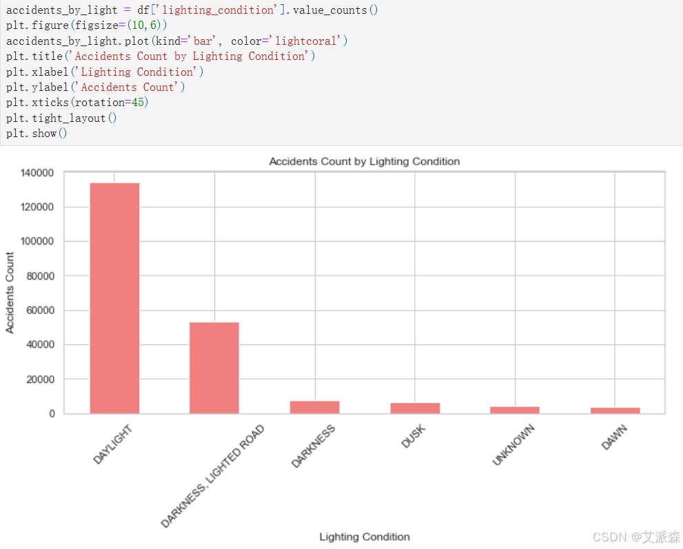
accidents_by_light = df['lighting_condition'].value_counts()
plt.figure(figsize=(10,6))
accidents_by_light.plot(kind='bar', color='lightcoral')
plt.title('Accidents Count by Lighting Condition')
plt.xlabel('Lighting Condition')
plt.ylabel('Accidents Count')
plt.xticks(rotation=45)
plt.tight_layout()
plt.show()
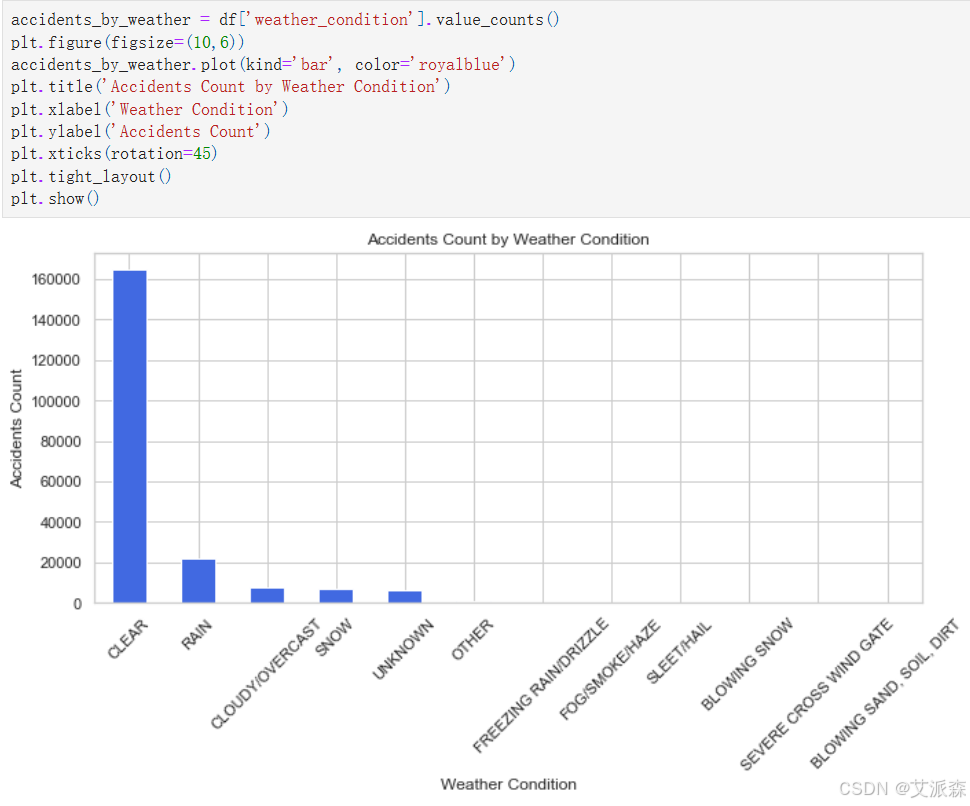
accidents_by_weather = df['weather_condition'].value_counts()
plt.figure(figsize=(10,6))
accidents_by_weather.plot(kind='bar', color='royalblue')
plt.title('Accidents Count by Weather Condition')
plt.xlabel('Weather Condition')
plt.ylabel('Accidents Count')
plt.xticks(rotation=45)
plt.tight_layout()
plt.show()
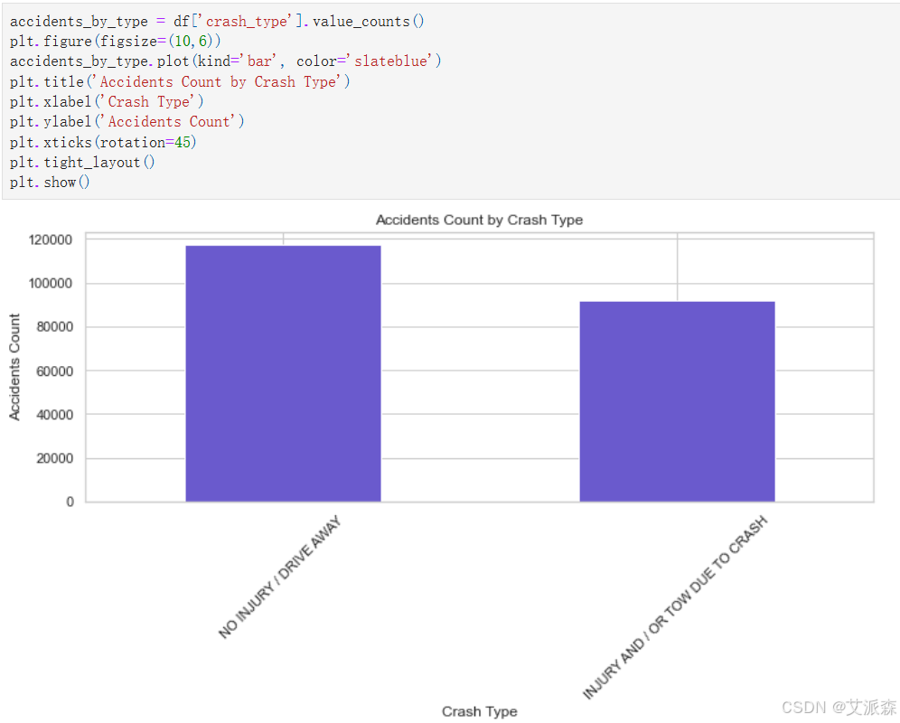
accidents_by_type = df['crash_type'].value_counts()
plt.figure(figsize=(10,6))
accidents_by_type.plot(kind='bar', color='slateblue')
plt.title('Accidents Count by Crash Type')
plt.xlabel('Crash Type')
plt.ylabel('Accidents Count')
plt.xticks(rotation=45)
plt.tight_layout()
plt.show()
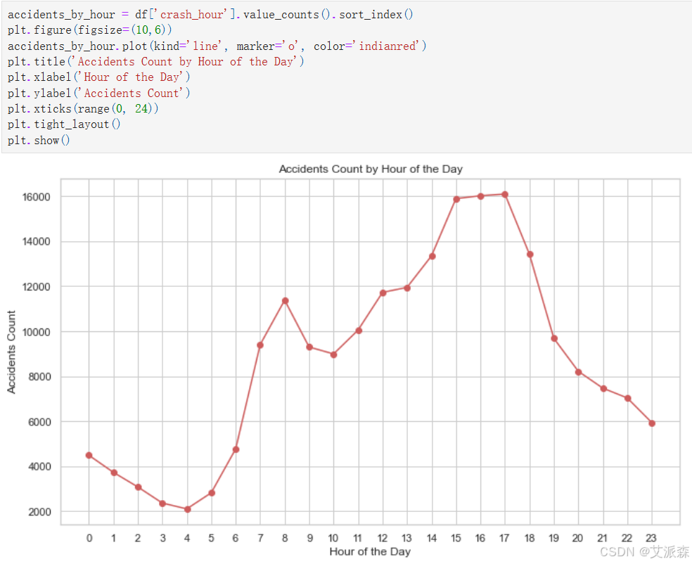
accidents_by_hour = df['crash_hour'].value_counts().sort_index()
plt.figure(figsize=(10,6))
accidents_by_hour.plot(kind='line', marker='o', color='indianred')
plt.title('Accidents Count by Hour of the Day')
plt.xlabel('Hour of the Day')
plt.ylabel('Accidents Count')
plt.xticks(range(0, 24))
plt.tight_layout()
plt.show()
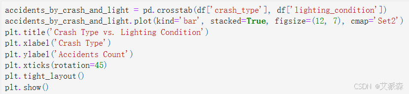
accidents_by_crash_and_light = pd.crosstab(df['crash_type'], df['lighting_condition'])
accidents_by_crash_and_light.plot(kind='bar', stacked=True, figsize=(12, 7), cmap='Set2')
plt.title('Crash Type vs. Lighting Condition')
plt.xlabel('Crash Type')
plt.ylabel('Accidents Count')
plt.xticks(rotation=45)
plt.tight_layout()
plt.show()
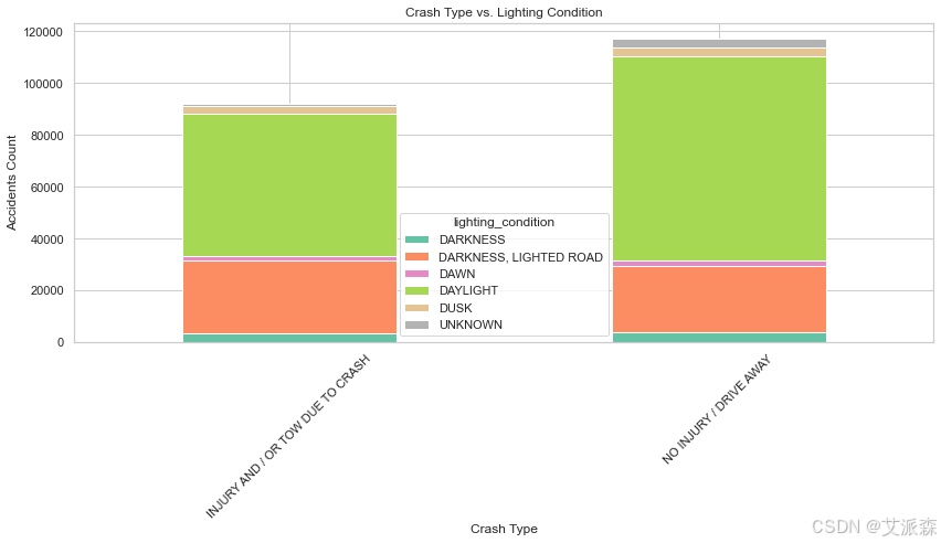
accidents_by_day = df['crash_day_of_week'].value_counts().sort_index()
plt.figure(figsize=(10,6))
accidents_by_day.plot(kind='bar', color='seagreen')
plt.title('Accidents Count by Day of the Week')
plt.xlabel('Day of the Week')
plt.ylabel('Accidents Count')
plt.xticks(ticks=range(7), labels=['Mon', 'Tue', 'Wed', 'Thu', 'Fri', 'Sat', 'Sun'])
plt.tight_layout()
plt.show()
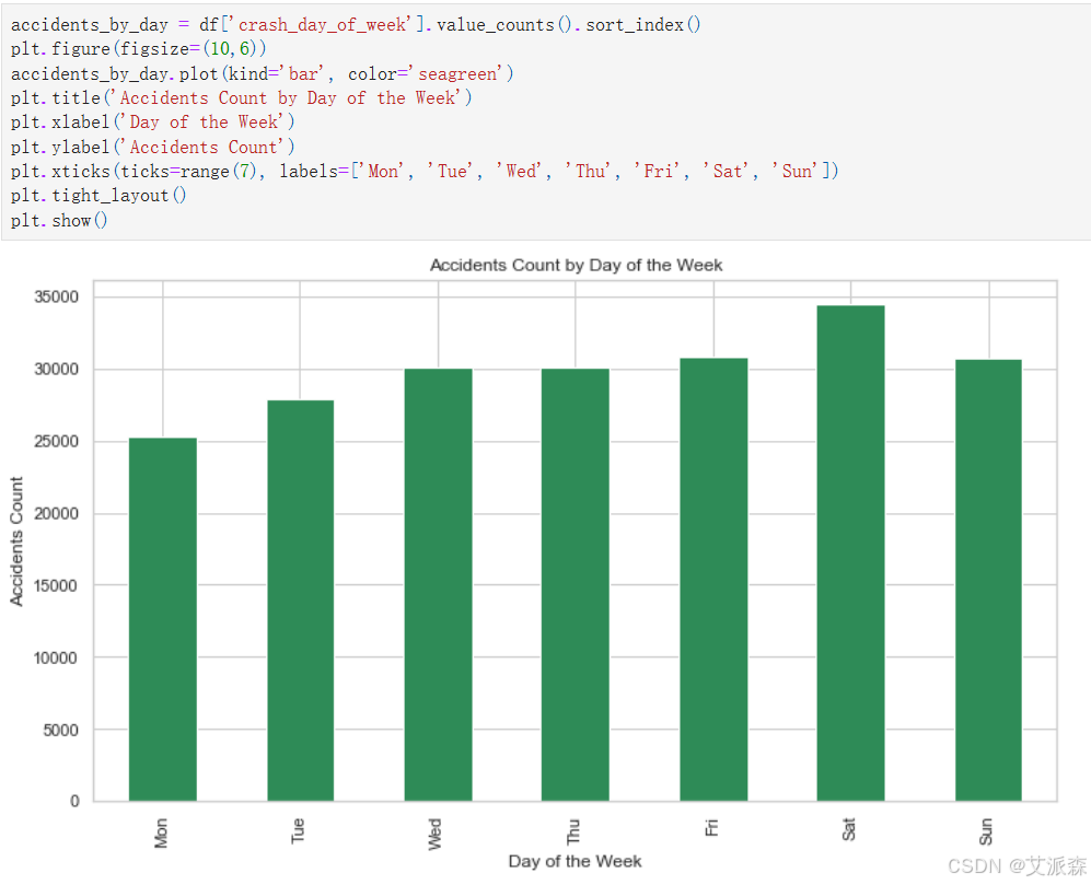
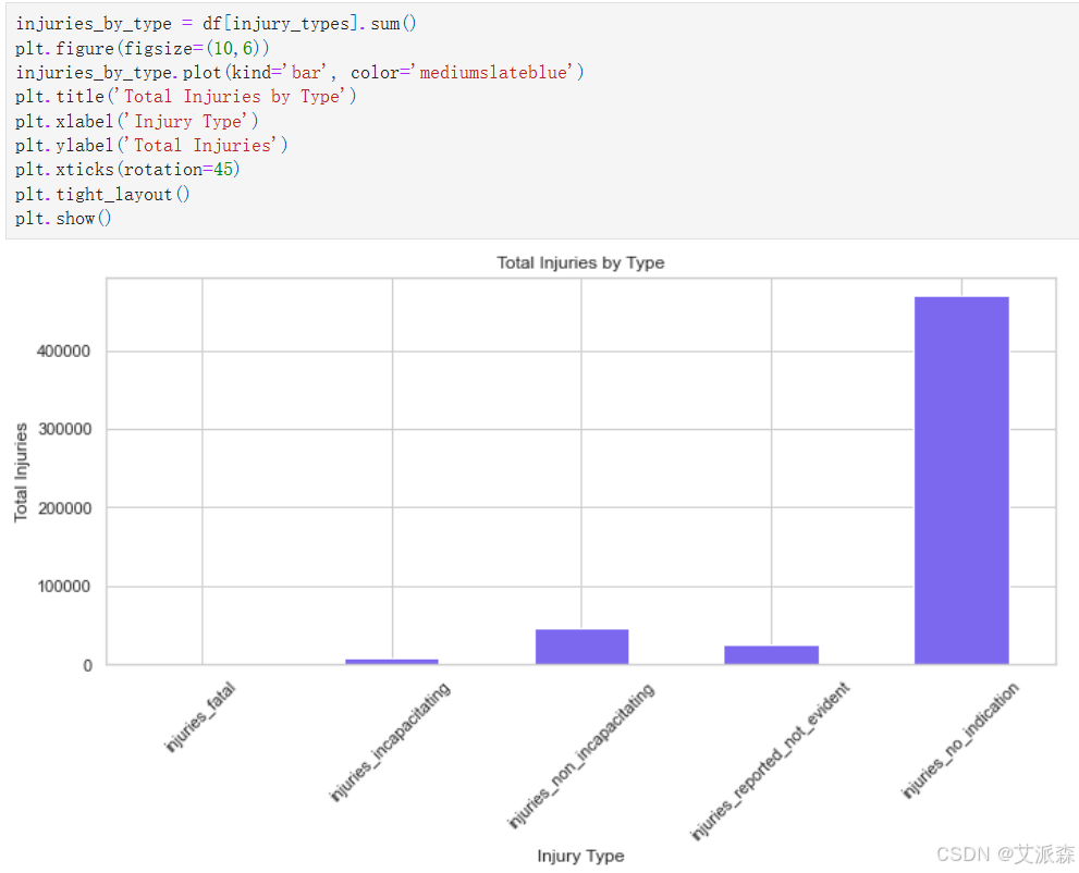
injuries_by_type = df[injury_types].sum()
plt.figure(figsize=(10,6))
injuries_by_type.plot(kind='bar', color='mediumslateblue')
plt.title('Total Injuries by Type')
plt.xlabel('Injury Type')
plt.ylabel('Total Injuries')
plt.xticks(rotation=45)
plt.tight_layout()
plt.show()
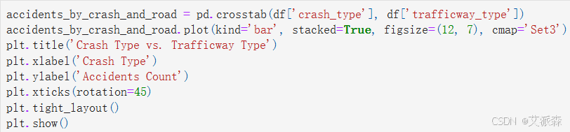
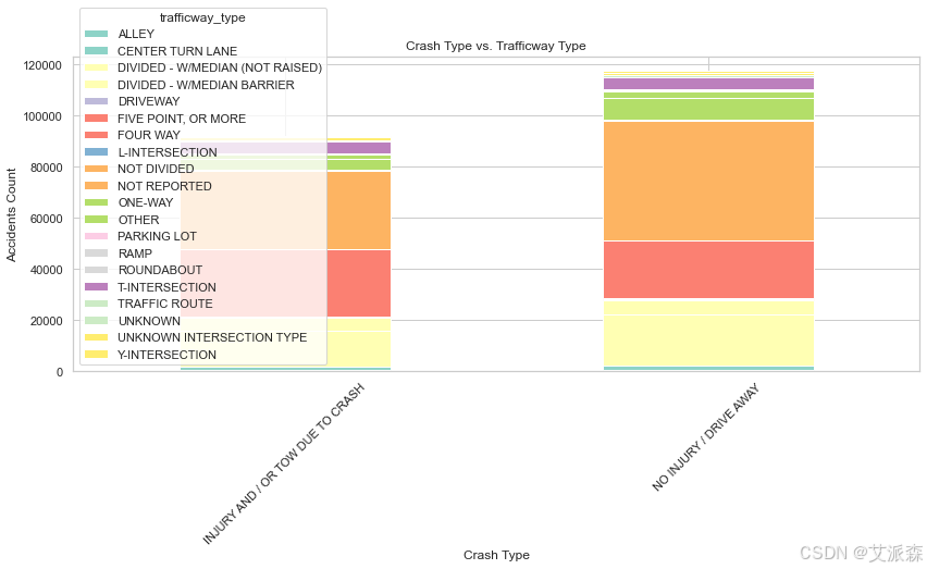
accidents_by_crash_and_road = pd.crosstab(df['crash_type'], df['trafficway_type'])
accidents_by_crash_and_road.plot(kind='bar', stacked=True, figsize=(12, 7), cmap='Set3')
plt.title('Crash Type vs. Trafficway Type')
plt.xlabel('Crash Type')
plt.ylabel('Accidents Count')
plt.xticks(rotation=45)
plt.tight_layout()
plt.show()
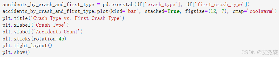
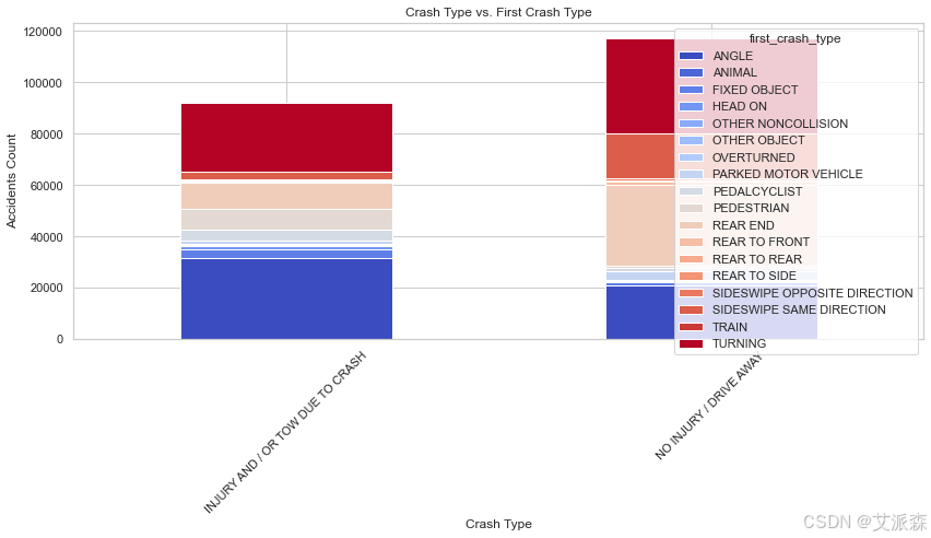
accidents_by_crash_and_first_type = pd.crosstab(df['crash_type'], df['first_crash_type'])
accidents_by_crash_and_first_type.plot(kind='bar', stacked=True, figsize=(12, 7), cmap='coolwarm')
plt.title('Crash Type vs. First Crash Type')
plt.xlabel('Crash Type')
plt.ylabel('Accidents Count')
plt.xticks(rotation=45)
plt.tight_layout()
plt.show()
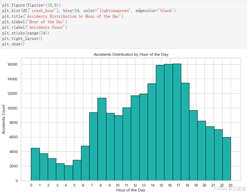
plt.figure(figsize=(10,6))
plt.hist(df['crash_hour'], bins=24, color='lightseagreen', edgecolor='black')
plt.title('Accidents Distribution by Hour of the Day')
plt.xlabel('Hour of the Day')
plt.ylabel('Accidents Count')
plt.xticks(range(24))
plt.tight_layout()
plt.show()
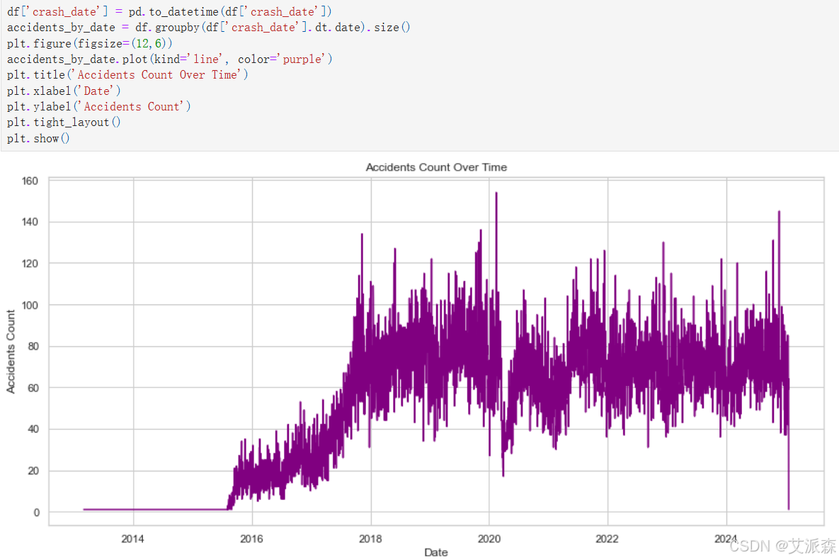
df['crash_date'] = pd.to_datetime(df['crash_date'])
accidents_by_date = df.groupby(df['crash_date'].dt.date).size()
plt.figure(figsize=(12,6))
accidents_by_date.plot(kind='line', color='purple')
plt.title('Accidents Count Over Time')
plt.xlabel('Date')
plt.ylabel('Accidents Count')
plt.tight_layout()
plt.show()
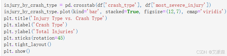
injury_by_crash_type = pd.crosstab(df['crash_type'], df['most_severe_injury'])
injury_by_crash_type.plot(kind='bar', stacked=True, figsize=(12,7), cmap='viridis')
plt.title('Injury Type vs. Crash Type')
plt.xlabel('Crash Type')
plt.ylabel('Total Injuries')
plt.xticks(rotation=45)
plt.tight_layout()
plt.show()
# 编码处理
label_encoders = {}
categorical_columns = df.select_dtypes(include=['object']).columns
for column in categorical_columns:
    original_values = df[column].unique()
    label_encoders[column] = LabelEncoder()
    df[column] = label_encoders[column].fit_transform(df[column])
    encoded_values = df[column].unique()
    decoded_values = label_encoders[column].inverse_transform(encoded_values)

df = df.drop(columns=['crash_date'])
df.head()
# 准备建模数据
X = df.drop(columns=['crash_type'])
y = df['crash_type']
# 拆分数据集为训练集和测试集
X_train, X_test, y_train, y_test = train_test_split(X, y, test_size=0.2, random_state=42)
# 随机森林模型
rf_model = RandomForestClassifier(n_estimators=100, random_state=42)
rf_model.fit(X_train, y_train)
y_pred = rf_model.predict(X_test)
print("Accuracy:", accuracy_score(y_test, y_pred))
print("Classification Report:")
print(classification_report(y_test, y_pred))
print("Confusion Matrix:")
print(confusion_matrix(y_test, y_pred))
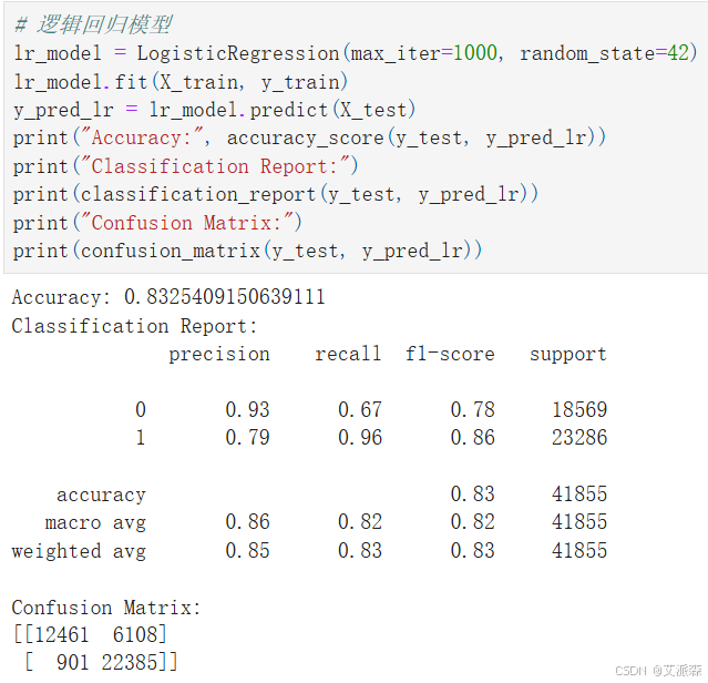
# 逻辑回归模型
lr_model = LogisticRegression(max_iter=1000, random_state=42)
lr_model.fit(X_train, y_train)
y_pred_lr = lr_model.predict(X_test)
print("Accuracy:", accuracy_score(y_test, y_pred_lr))
print("Classification Report:")
print(classification_report(y_test, y_pred_lr))
print("Confusion Matrix:")
print(confusion_matrix(y_test, y_pred_lr))
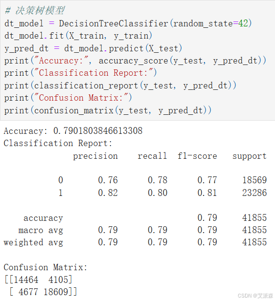
# 决策树模型
dt_model = DecisionTreeClassifier(random_state=42)
dt_model.fit(X_train, y_train)
y_pred_dt = dt_model.predict(X_test)
print("Accuracy:", accuracy_score(y_test, y_pred_dt))
print("Classification Report:")
print(classification_report(y_test, y_pred_dt))
print("Confusion Matrix:")
print(confusion_matrix(y_test, y_pred_dt))
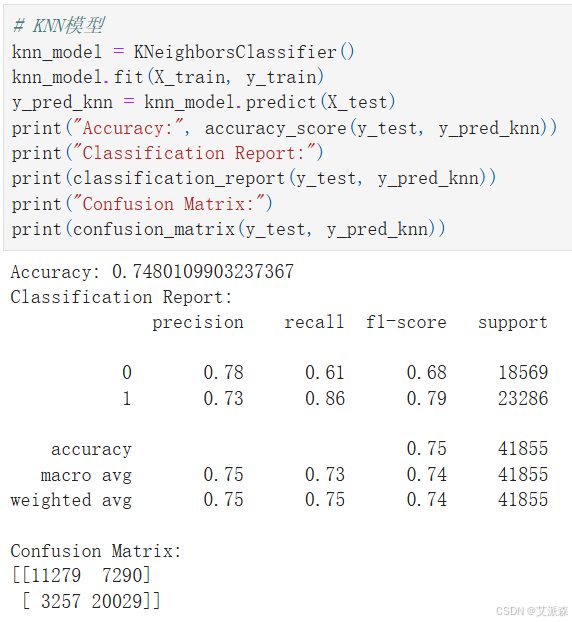
# KNN模型
knn_model = KNeighborsClassifier()
knn_model.fit(X_train, y_train)
y_pred_knn = knn_model.predict(X_test)
print("Accuracy:", accuracy_score(y_test, y_pred_knn))
print("Classification Report:")
print(classification_report(y_test, y_pred_knn))
print("Confusion Matrix:")
print(confusion_matrix(y_test, y_pred_knn))
models = ['Random Forest', 'Logistic Regression', 'Decision Tree','KNN']
accuracies = [accuracy_score(y_test, rf_model.predict(X_test)),
              accuracy_score(y_test, lr_model.predict(X_test)),
              accuracy_score(y_test, dt_model.predict(X_test)),
              accuracy_score(y_test, knn_model.predict(X_test)),
             ]

model_comparison = pd.DataFrame({
    'Model': models,
    'Accuracy': accuracies
})

print(model_comparison)
# 特征重要性
Feature_importances = rf_model.feature_importances_
sorted_indices = np.argsort(Feature_importances)

plt.figure(figsize=(10, 5))
plt.barh(np.array(X.columns)[sorted_indices], Feature_importances[sorted_indices], color=plt.cm.rainbow(np.linspace(0, 1, len(Feature_importances))), alpha=0.7)
plt.title("Feature Importances - Random Forest")
plt.xlabel("Importance")
plt.tight_layout()
plt.show()

资料获取，更多粉丝福利，关注下方公众号获取

在这里插入图片描述