【Kaggle】AMEX信用违约预测比赛总结

American Express - Default Prediction（AMEX）https://www.kaggle.com/competitions/amex-default-prediction/overview     —— 2022/8/25 已结束

• 大规模表格型数据
• 欺诈预测

零、数据描述

本次竞赛的目的是根据客户的每月客户资料预测客户未来不偿还信用卡余额的概率。目标二元变量是通过观察最新信用卡对账单后18个月的表现窗口来计算的，如果客户在最新对账单日期后120天内未支付到期金额，则视为违约事件。

数据集包含每个客户在每个报表日期的聚合配置文件特征。功能被匿名化和规范化，并分为以下一般类别：

• D_* = Delinquency variables
• S_* = Spend variables
• P_* = Payment variables
• B_* = Balance variables
• R_* = Risk variables

文件包含：

• train_data.csv - training data with multiple statement dates per customer_ID
• train_labels.csv - target label for each customer_ID
• test_data.csv - corresponding test data; your objective is to predict the target label for each customer_ID
• sample_submission.csv - a sample submission file in the correct format

AMEX EDA which makes sense ⭐️⭐️⭐️⭐️⭐️ | Kaggle

一、数据探索

1. 数据中的噪点

The data has random uniform noise added | Kaggle

对数据B_*，金钱数据的分布应该是离散并间隔$0.01。但是观察到 (1, 1.01)不止单一值，

 并且99.9%的值在B_2特征上唯一，不符合银行中钱的分布，可以判断有噪点（±0.01）被加入。

处理方案：

Integer columns in the data：0.01 wide bin，找到整数乘数使数据离散

2. 逾期有关特征

Deanonymized days overdue feat (AMEX) | Kaggle

D_39特征

 3. 缺失值分布

Understanding NA values in AMEX competition | Kaggle

• Some NA appears only on the first observation for each customer! So for this feature cluster NA represents fresh credit card accounts with probably zero balance
• 6879 NA in the mix which may or may not be missing at random

二、数据预处理

减少内存：

• 数据噪点清除：float -> int，50GB -> 5GB
• 数据存储格式：Parquet, 50G->10G；或者feather文件

加速读取：

• CUPY/CUDF：GPU读取数据

缺失值：

Raddar：两种类型缺失值，一种随机缺失，另一种NA只出现在每个客户的第一次观察中，对于此，NA表示可能为零余额的新信用卡帐户！

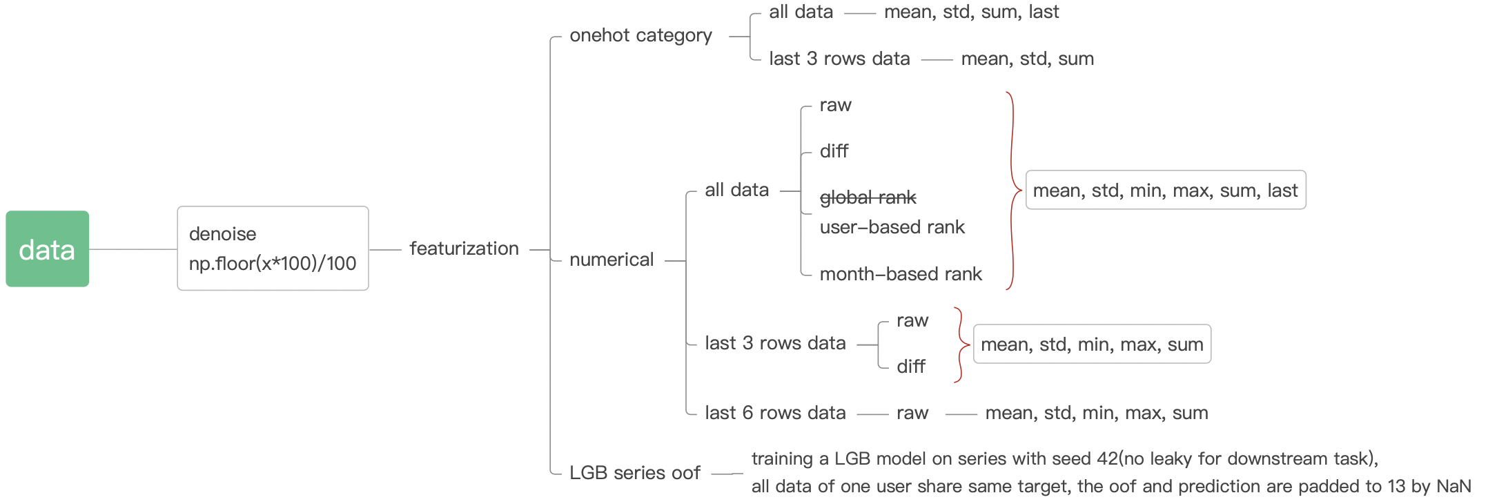
三、特征工程

1. Diff

def get_difference(data, num_features):
    df1 = []
    customer_ids = []
    for customer_id, df in tqdm(data.groupby(['customer_ID'])):
        # Get the differences
        diff_df1 = df[num_features].diff(1).iloc[[-1]].values.astype(np.float32)
        # Append to lists
        df1.append(diff_df1)
        customer_ids.append(customer_id)
    # Concatenate
    df1 = np.concatenate(df1, axis = 0)
    # Transform to dataframe
    df1 = pd.DataFrame(df1, columns = [col + '_diff1' for col in df[num_features].columns])
    # Add customer id
    df1['customer_ID'] = customer_ids
    return df1

2. Lag

Lag Features Are All You Need | Kaggle

"Lag" fearures: to capture the change over time about each client I calculated two features for every first, last pair:

• Last - First: The change since we first see the client to the last time we see the client.
• Last / First: The fractional difference since we first see the client to the last time we see the client.

# Lag Features
for col in test_num_agg:
    if 'last' in col and col.replace('last', 'first') in test_num_agg:
        test_num_agg[col + '_lag_sub'] = test_num_agg[col] - test_num_agg[col.replace('last', 'first')]
        test_num_agg[col + '_lag_div'] = test_num_agg[col] / test_num_agg[col.replace('last', 'first')]

test_cat_agg = test.groupby("customer_ID")[cat_features].agg(['count', 'first', 'last','nunique'])
test_cat_agg.columns = ['_'.join(x) for x in test_cat_agg.columns]
test_cat_agg.reset_index(inplace = True)

Lag_1 & last difference: The difference between last value and the lag1

Average & last difference: The difference between last value and the average

3. Rank

Learning to rank - time related features | Kaggle

each customer has N months of history observed (N = 1,...,13).

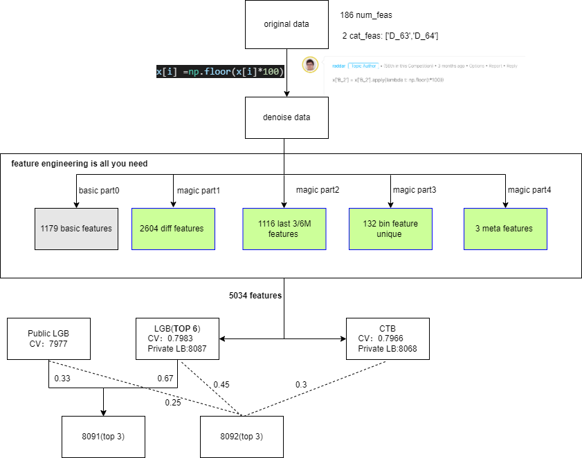
四、模型代码

XGBoost | LGBT | DART | LightAutoML

• LGBM DART：Amex LGBM Dart CV 0.7977 | Kaggle
• XGBoost：XGBoost Starter - [0.793] | Kaggle

TabNet | GRU | Transformer

• TabNet：AMEX TabNetClassifier + Feature Eng [0.791] | Kaggle

!pip install pytorch-tabnet -q

from pytorch_tabnet.tab_model import TabNetClassifier
from pytorch_tabnet.metrics import Metric

# using amex metric to evaluate tabnet
class Amex_tabnet(Metric):
    
  def __init__(self):
    self._name = 'amex_tabnet'
    self._maximize = True

  def __call__(self, y_true, y_pred):
    amex = amex_metric_numpy(y_true, y_pred[:, 1])
    return max(amex, 0.)


model = TabNetClassifier(n_d = 32, #决定输出的隐藏层神经元个数
                         n_a = 64, #决定下一决策步特征选择的隐藏层神经元个数
                         n_steps = 3, #决策步的个数。可理解为决策树中分裂结点的次数
                         gamma = 1.3, #决定历史所用特征在当前决策步的特征选择阶段的权重
                         cat_idxs = cat_index,                                 
                         n_independent = 2,
                         n_shared = 2,
                         momentum = 0.02,
                         clip_value = None,
                         lambda_sparse = 1e-3, #稀疏正则项权重，对特征选择添加约束
                         optimizer_fn = torch.optim.Adam,
                         scheduler_fn = torch.optim.lr_scheduler.CosineAnnealingLR,
                         scheduler_params = {"T_max" : 6},
                         mask_type = 'sparsemax',
                         seed = CFG.seed)

model.fit(np.array(X_train),
          np.array(y_train.values.ravel()),
          eval_set = [(np.array(X_valid), np.array(y_valid.values.ravel()))],
          max_epochs = 50,
          patience = 10, # 在验证集上早停次数
          batch_size = 2048,
          eval_metric = ['auc', 'accuracy', Amex_tabnet])

• GRU：TensorFlow GRU Starter - [0.790] | Kaggle

'''FE'''
    # PAD ROWS SO EACH CUSTOMER HAS 13 ROWS
    if PAD_CUSTOMER_TO_13_ROWS:
        tmp = train[['customer_ID']].groupby('customer_ID').customer_ID.agg('count')
        more = cupy.array([],dtype='int64') 
        for j in range(1,13):
            i = tmp.loc[tmp==j].index.values
            more = cupy.concatenate([more,cupy.repeat(i,13-j)])
        df = train.iloc[:len(more)].copy().fillna(0)
        df = df * 0 - 1 #pad numerical columns with -1
        df[CATS] = (df[CATS] * 0).astype('int8') #pad categorical columns with 0
        df['customer_ID'] = more
        train = cudf.concat([train,df],axis=0,ignore_index=True)


# SIMPLE GRU MODEL
def build_model():
    
    # INPUT - FIRST 11 COLUMNS ARE CAT, NEXT 177 ARE NUMERIC
    inp = tf.keras.Input(shape=(13,188))
    embeddings = []
    for k in range(11):
        emb = tf.keras.layers.Embedding(10,4)
        embeddings.append( emb(inp[:,:,k]) )
    x = tf.keras.layers.Concatenate()([inp[:,:,11:]]+embeddings)
    
    # SIMPLE RNN BACKBONE
    x = tf.keras.layers.GRU(units=128, return_sequences=False)(x)
    x = tf.keras.layers.Dense(64,activation='relu')(x)
    x = tf.keras.layers.Dense(32,activation='relu')(x)
    
    # OUTPUT
    x = tf.keras.layers.Dense(1,activation='sigmoid')(x)
    
    # COMPILE MODEL
    model = tf.keras.Model(inputs=inp, outputs=x)
    opt = tf.keras.optimizers.Adam(learning_rate=0.001)
    loss = tf.keras.losses.BinaryCrossentropy()
    model.compile(loss=loss, optimizer = opt)
    
    return model

# CUSTOM LEARNING SCHEUDLE
def lrfn(epoch):
    lr = [1e-3]*5 + [1e-4]*2 + [1e-5]*1
    return lr[epoch]
LR = tf.keras.callbacks.LearningRateScheduler(lrfn, verbose = False)


# BUILD AND TRAIN MODEL
        K.clear_session()
        model = build_model()
        h = model.fit(X_train,y_train, 
                      validation_data = (X_valid,y_valid),
                      batch_size=512, epochs=8, verbose=VERBOSE,
                      callbacks = [LR])

Rank Ensemble

AMEX Rank Ensemble | Kaggle

from scipy.stats import rankdata

for df, weight in zip(dfs, weights):
    submit['prediction'] += (rankdata(df['prediction'])/df.shape[0]) * weight

五、解决方案

1st Solution

1st solution(update github code)

2nd Solution

2nd place solution - team JuneHomes (writeup)

3rd Solution

10th Place Solution

XGB with Autoregressive RNN features

10th Place Solution: XGB with Autoregressive RNN features

11th Place Solution

11th Place Solution (LightGBM with meta features)

• Meta features (most important features!)
  • how to make
    1. Train_labels are assigned to train data (before aggregation by cid) and train model.
    2. Make oof prediction for train data.
    3. Aggregate oof prediction by time period.
  • Using this feature, I reached 0.800 PublicLB from 0.799 PublicLB in single model.
  • Referring to the DSB2019's 2nd place solution method.
    • 2019 Data Science Bowl | Kaggle

14th Solution

NN Transformer using LGBM Knowledge Distillation

14th Place Gold – NN Transformer using LGBM Knowledge Distillation

25th Solution

SequentialEncoder

25th place solution

---

American Express - Default Prediction | Kaggle