


目录
PyTorch——开源的Python机器学习库
一、前言
首先感谢所有点开本文的朋友们!基于PyTorch的深度学习实战可能要告一段落了。本想着再写几篇关于PyTorch神经网络深度学习的文章来着,可无奈项目时间紧任务重,要求短时间内出图并做好参数拟合。所以只得转战Matlab编程,框架旧就旧吧,无所谓了 (能出结果就行) 。
往期回顾:
[深度学习实战]基于PyTorch的深度学习实战(上)[变量、求导、损失函数、优化器]
[深度学习实战]基于PyTorch的深度学习实战(中)[线性回归、numpy矩阵的保存、模型的保存和导入、卷积层、池化层]
二、Mnist手写数字图像识别
一个典型的神经网络的训练过程大致分为以下几个步骤:
(1)首先定义神经网络的结构,并且定义各层的权重参数的规模和初始值。
(2)然后将输入数据分成多个批次输入神经网络。
(3)将输入数据通过整个网络进行计算。
(4)每次迭代根据计算结果和真实结果的差值计算损失。
(5)根据损失对权重参数进行反向求导传播。
(6)更新权重值,更新过程使用下面的公式:
weight = weight + learning_rate * gradient。其中 weight 是上一次的权重值,learning_rate 是学习步长,gradient 是求导值。
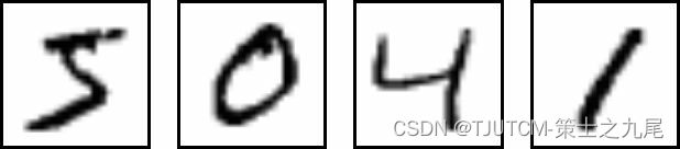
下面我们还是以经典的图像识别卷积网络作为例子来学习 pytorch 的用法。选择一个较小的数据集进行训练,这里我们选择 mnist 手写识别数据集,该数据集是 0-9 个数字的训练数据和测试数据,训练数据 60000 张图片,测试数据 10000 张图片。每张图片是 28×28 像素大小的单通道黑白图片,这样读到内存数据组就是 28 * 28 * 1 大小。这里的 28 * 28 是宽度和高度的像素数量,1 是图像通道数据(如果是彩色图像就是 3 道路,内存数据为 28 * 28 * 3 大小)。
我们先看看样本图像的模样:
好,下一步我们构建一个简单的卷积神经网络模型,这个模型的输入是图片,输出是 0-9 的数字,这是一个典型的监督式分类神经网络。
2.1 加载数据
这里我们不打算下载原始的图像文件然后通过 opencv 等图像库读取到数组,而是直接下载中间数据。当然读者也可以下载原始图像文件从头开始装载数据,这样对整个模型会有更深刻的体会。
我们用 mnist 数据集作例子,下载方法有两种:
2.1.1 下载地址
http://yann.lecun.com/exdb/mnist/。一共四个文件:
train-images-idx3-ubyte.gz: training set images (9912422 bytes)
train-labels-idx1-ubyte.gz: training set labels (28881 bytes)
t10k-images-idx3-ubyte.gz: test set images (1648877 bytes)
t10k-labels-idx1-ubyte.gz: test set labels (4542 bytes)
这些文件中是已经处理过的数组数据,通过numpy的相关方法读取到训练数据集和测试数据集数组中。注意调用 load_mnist 方法之前先解压上述四个文件。
from __future__ import print_function
import os
import struct
import numpy as np
def load_mnist(path, kind='train'):
labels_path = os.path.join(path, '%s-labels.idx1-ubyte' % kind)
images_path = os.path.join(path, '%s-images.idx3-ubyte' % kind)
with open(labels_path, 'rb') as lbpath:
magic, n = struct.unpack('>II', lbpath.read(8))
labels = np.fromfile(lbpath, dtype=np.uint8)
with open(images_path, 'rb') as imgpath:
magic, num, rows, cols = struct.unpack(">IIII", imgpath.read(16))
images = np.fromfile(imgpath, dtype=np.uint8).reshape(len(labels), 784)
return images, labels
X_train, y_train = load_mnist('./data', kind='train')
print('Rows: %d, columns: %d' % (X_train.shape[0], X_train.shape[1]))
X_test, y_test = load_mnist('./data', kind='t10k')
print('Rows: %d, columns: %d' % (X_test.shape[0], X_test.shape[1]))
显示结果:
D:\AI>python mnist_cnn.py
Rows: 60000, columns: 784
Rows: 10000, columns: 784
我们看到训练数据的行数是 60000,表示 60000 张图片,列是 784,表示 28281=784 个像素,测试数据是 10000 张图片,在后面构建卷积模型时,要先将 784 个像素的列 reshape 成 28281 维度。
例如:
image1 = X_train[1]
image1 = image1.astype('float32')
image1 = image1.reshape(28,28,1)
我们还可以将这些图像数组导出为 jpg 文件,比如下面的代码:
import cv2
cv2.imwrite('1.jpg',image1)
当前目录下的 1.jpg 文件都是我们导出的图像文件了。
图像的显示:
import cv2
import numpy as np
img = cv2.imread("C:\lena.jpg")
cv2.imshow("lena",img)
cv2.waitKey(10000)
2.1.2 用 numpy 读取 mnist.npz
可以直接从亚马逊下载文件:
https://s3.amazonaws.com/imgdatasets/mnist.npz
Mnist.npz 是一个 numpy 数组文件。如果下载的是 mnist.npz.gz 文件,则用 gunzip mnist.npz.gz 先解压成 mnist.npz,然后再处理。也可以调用 keras 的方法来下载:
from keras.datasets import mnist
(x_train, y_train), (x_test, y_test) = mnist.load_data()
通过 mnist.load_data() 下载的 mnist.npz 会放在当前用户的 .keras 目录中。路径名称:
~/.keras/datasets/mnist.npz
然后调用 numpy 来加载 mnist.npz。
示例代码:
import numpy as np
class mnist_data(object):
def load_npz(self,path):
f = np.load(path)
for i in f:
print i
x_train = f['trainInps']
y_train = f['trainTargs']
x_test = f['testInps']
y_test = f['testTargs']
f.close()
return (x_train, y_train), (x_test, y_test)
a = mnist_data()
(x_train, y_train), (x_test, y_test) = a.load_npz('D:/AI/torch/data/mnist.npz')
print ("train rows:%d,test rows:%d"% (x_train.shape[0], x_test.shape[0]))
print("x_train shape",x_train.shape)
print("y_train shape",y_train.shape )
结果:
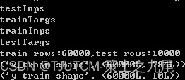
一共 60000 张训练图片,10000 张测试图片。训练图像的大小 784 个像素,也就是 1 通道的 28*28 的手写图片。标签是长度为 10 的 (0,1) 向量,表示 0-9 是个数字。例如数字 1 就表示为 [0,1,0,0,0,0,0,0,0,0]。
让我们打印出第一张图片的截图和标签。代码如下:
tt=x_train[1]
tt=tt.astype('float32')
image = tt.reshape(28,28,1)
cv2.imwrite("001.png",image)
print("tt label:",y_train[1])


标签为 [0,0,0,1,0,0,0,0,0,0]。
2.2 定义卷积模型
这一步我们定义自己的卷积模型,对于 28 * 28 的数组,我们定义 (5,5) 的卷积核大小比较合适,卷积核的大小可根据图像大小灵活设置,比如 (3,3),(5,5),(9,9)等。一般卷积核的大小是奇数。
输入数据首先连接 1 个卷积层加 1 个池化层,conv1 和 pool1,假设我们定义 conv1 的神经元数目为 10,卷积核大小 (5,5),定义 pool1 的大小 (2,2),意思将 2 * 2区域共 4 个像素统计为 1 个像素,这样这层数据量减少 4 倍。这时候输出图像大小为 (28-5+1)/2=12。输出数据维度(10,12,12)。
接着再来一次卷积池化,连接 1 个卷积层加 1 个池化层,conv2 和 pool2,假设我们定义 conv2 的神经元数目为 20,卷积核大小 (5,5),定义pool2的大小 (2,2),意思将 2*2 区域共 4 个像素统计为 1 个像素,这样这层数据量减少 4 倍。这时候输出图像大小为 (12-5+1)/2=4。输出数据维度 (20,4,4)。
然后接一个 dropout 层,设置 dropout=0.2,随机抛弃部分数据。
最后连续接两个全连接层,第一个全连接层 dense1 输入维度 20 * 4 * 4,输出 320,第二个全连接层 dense1 输入维度 60,输出 10。
模型定义的 pytorch 代码如下:
class Net(nn.Module):
def __init__(self):
super(Net, self).__init__()
self.conv1 = nn.Conv2d(1, 10, kernel_size=5)
self.conv2 = nn.Conv2d(10, 20, kernel_size=5)
self.conv2_drop = nn.Dropout2d()
self.fc1 = nn.Linear(320, 60)
self.fc2 = nn.Linear(60, 10)
def forward(self, x):
x = F.relu(F.max_pool2d(self.conv1(x), 2))
x = F.relu(F.max_pool2d(self.conv2_drop(self.conv2(x)), 2))
x = x.view(-1, 320)
x = F.relu(self.fc1(x))
x = F.dropout(x, training=self.training)
x = self.fc2(x)
return F.log_softmax(x)
model = Net()
print(model)
注解:nn.Conv2d(1, 10, kernel_size=5) 是指将 1 通道的图像数据的输入卷积成 10 个神经元,这 1 个通道跟 10 个神经元都建立连接,然后神经网络对每个连接计算出不同的权重值,某个神经元上的权重值对原图卷积来提取该神经元负责的特征。这个过程是神经网络自动计算得出的。
那么 nn.Conv2d(10, 20, kernel_size=5) 是指将 10 通道的图像数据的输入卷积成 20 个神经元,同样的,这 10 个通道会和 20 个神经元的每一个建立连接,那么10 个通道如何卷积到 1 个通道呢?一般是取 10 个通道的平均值作为最后的结果。
执行该脚本,将卷积模型的结构打印出来:
[root@iZ25ix41uc3Z ai]# python mnist_torch.py
Net (
(conv1): Conv2d(1, 10, kernel_size=(5, 5), stride=(1, 1))
(conv2): Conv2d(10, 20, kernel_size=(5, 5), stride=(1, 1))
(conv2_drop): Dropout2d (p=0.5)
(fc1): Linear (320 -> 50)
(fc2): Linear (50 -> 10)
)
2.3 开始训练
数据准备好,模型建立好,下面根据神经网络的三部曲,就是选择损失函数和梯度算法对模型进行训练了。
损失函数通俗讲就是计算模型的计算结果和真实结果之间差异性的函数,典型的如距离的平方和再开平方,对于图像分类来说,我们取的损失函数是:
F.log_softmax(x)
在神经网络的训练过程中,我们使用 loss.backward() 来反向传递修正,反向修正就是根据计算和真实结果的差值(就是损失)来反向逆传播修正各层的权重参数,修正之后的结果保存在 .grad 中,因此每轮迭代执行 loss.backward() 的时候要先对 .grad 清零。
model.zero_grad()
print('conv1.bias.grad before backward')
print(model.conv1.bias.grad)
loss.backward()
print('conv1.bias.grad after backward')
print(model.conv1.bias.grad)
优化算法一般是指迭代更新权重参数的梯度算法,这里我们选择随机梯度算法 SGD。
SGD 的算法如下:
weight = weight - learning_rate * gradient
可以用一段简单的 python 脚本模拟这个 SGD 的过程:
learning_rate = 0.01
for f in model.parameters():
f.data.sub_(f.grad.data * learning_rate)
pytorch 中含有其他的优化算法,如 Nesterov-SGD, Adam, RMSProp 等。
它们的用法和 SGD 基本类似,这里就不一一介绍了。
训练代码如下:
import torch.optim as optim
input = Variable(torch.randn(1, 1, 32, 32))
out = model(input)
print(out)
# create your optimizer
optimizer = optim.SGD(model.parameters(), lr=0.01)
# in your training loop:
optimizer.zero_grad() # zero the gradient buffers
output = model(input)
loss = criterion(output, target)
loss.backward()
optimizer.step() # Does the update
2.4 完整代码
最后的代码如下所示,这里我们做了一点修改,每次迭代完会将模型参数保存到文件,下次再次执行脚本会自动加载上次迭代后的数据。整个完整的代码如下:
'''
Trains a simple convnet on the MNIST dataset.
'''
from __future__ import print_function
import os
import struct
import numpy as np
import torch
import torch.nn as nn
import torch.nn.functional as F
import torch.optim as optim
from torch.autograd import Variable
def load_mnist(path, kind='train'):
"""Load MNIST data from `path`"""
labels_path = os.path.join(path, '%s-labels.idx1-ubyte' % kind)
images_path = os.path.join(path, '%s-images.idx3-ubyte' % kind)
with open(labels_path, 'rb') as lbpath:
magic, n = struct.unpack('>II', lbpath.read(8))
labels = np.fromfile(lbpath, dtype=np.uint8)
with open(images_path, 'rb') as imgpath:
magic, num, rows, cols = struct.unpack(">IIII", imgpath.read(16))
images = np.fromfile(imgpath, dtype=np.uint8).reshape(len(labels), 784)
return images, labels
X_train, y_train = load_mnist('./data', kind='train')
print("shape:",X_train.shape)
print('Rows: %d, columns: %d' % (X_train.shape[0], X_train.shape[1]))
X_test, y_test = load_mnist('./data', kind='t10k')
print('Rows: %d, columns: %d' % (X_test.shape[0], X_test.shape[1]))
batch_size = 100
num_classes = 10
epochs = 2
# input image dimensions
img_rows, img_cols = 28, 28
x_train= X_train
x_test=X_test
if 'channels_first' == 'channels_first':
x_train = x_train.reshape(x_train.shape[0], 1, img_rows, img_cols)
x_test = x_test.reshape(x_test.shape[0], 1, img_rows, img_cols)
input_shape = (1, img_rows, img_cols)
else:
x_train = x_train.reshape(x_train.shape[0], img_rows, img_cols, 1)
x_test = x_test.reshape(x_test.shape[0], img_rows, img_cols, 1)
input_shape = (img_rows, img_cols, 1)
x_train = x_train.astype('float32')
x_test = x_test.astype('float32')
x_train /= 255
x_test /= 255
print('x_train shape:', x_train.shape)
print(x_train.shape[0], 'train samples')
print(x_test.shape[0], 'test samples')
num_samples=x_train.shape[0]
print("num_samples:",num_samples)
'''
build torch model
'''
class Net(nn.Module):
def __init__(self):
super(Net, self).__init__()
self.conv1 = nn.Conv2d(1, 10, kernel_size=5)
self.conv2 = nn.Conv2d(10, 20, kernel_size=5)
self.conv2_drop = nn.Dropout2d()
self.fc1 = nn.Linear(320, 50)
self.fc2 = nn.Linear(50, 10)
def forward(self, x):
x = F.relu(F.max_pool2d(self.conv1(x), 2))
x = F.relu(F.max_pool2d(self.conv2_drop(self.conv2(x)), 2))
x = x.view(-1, 320)
x = F.relu(self.fc1(x))
x = F.dropout(x, training=self.training)
x = self.fc2(x)
return F.log_softmax(x)
model = Net()
if os.path.exists('mnist_torch.pkl'):
model = torch.load('mnist_torch.pkl')
print(model)
'''
trainning
'''
optimizer = optim.SGD(model.parameters(), lr=0.01, momentum=0.5)
#loss=torch.nn.CrossEntropyLoss(size_average=True)
def train(epoch,x_train,y_train):
num_batchs = num_samples/ batch_size
model.train()
for k in range(num_batchs):
start,end = k*batch_size,(k+1)*batch_size
data, target = Variable(x_train[start:end],requires_grad=False), Variable(y_train[optimizer.zero_grad()
output = model(data)
loss = F.nll_loss(output, target)
loss.backward()
optimizer.step()
if k % 10 == 0:
print('Train Epoch: {} [{}/{} ({:.0f}%)]\tLoss: {:.6f}'.format(
epoch, k * len(data), num_samples,
100. * k / num_samples, loss.data[0]))
torch.save(model, 'mnist_torch.pkl')
'''
evaludate
'''
def test(epoch):
model.eval()
test_loss = 0
correct = 0
if 2>1:
data, target = Variable(x_test, volatile=True), Variable(y_test)
output = model(data)
test_loss += F.nll_loss(output, target).data[0]
pred = output.data.max(1)[1] # get the index of the max log-probability
correct += pred.eq(target.data).cpu().sum()
test_loss = test_loss
test_loss /= len(x_test) # loss function already averages over batch size
print('\nTest set: Average loss: {:.4f}, Accuracy: {}/{} ({:.0f}%)\n'.format(
test_loss, correct, len(x_test),
100. * correct / len(x_test)))
x_train=torch.from_numpy(x_train).float()
x_test=torch.from_numpy(x_test).float()
y_train=torch.from_numpy(y_train).long()
y_test=torch.from_numpy(y_test).long()
for epoch in range(1,epochs):
train(epoch,x_train,y_train)
test(epoch)
2.5 验证结果
2 次迭代后:Test set: Average loss: 0.3419, Accuracy: 9140/10000 (91%)
3 次迭代后:Test set: Average loss: 0.2362, Accuracy: 9379/10000 (94%)
4 次迭代后:Test set: Average loss: 0.2210, Accuracy: 9460/10000 (95%)
5 次迭代后:Test set: Average loss: 0.1789, Accuracy: 9532/10000 (95%)
顺便说一句,pytorch 的速度比 keras 确实要快很多,每次迭代几乎 1 分钟内就完成了,确实很不错!
2.6 修改参数
我们把卷积层的神经元个数重新设置一下,第一层卷积加到 32 个,第二层卷积神经元加到 64 个。则新的模型为下面的组织:
{
(conv1): Conv2d(1, 32, kernel_size=(5, 5), stride=(1, 1))
(conv2): Conv2d(32, 64, kernel_size=(5, 5), stride=(1, 1))
(conv2_drop): Dropout2d (p=0.5)
(fc1): Linear (1024 -> 100)
(fc2): Linear (100 -> 10)
)
然后同样的步骤我们跑一遍看看结果如何,这次明显慢了很多,但看的出来准确度也提高了一些:
第 1 次迭代:Test set: Average loss: 0.3159, Accuracy: 9038/10000 (90%)
第 2 次迭代:Test set: Average loss: 0.1742, Accuracy: 9456/10000 (95%)
第 3 次迭代:Test set: Average loss: 0.1234, Accuracy: 9608/10000 (96%)
第 4 次迭代:Test set: Average loss: 0.1009, Accuracy: 9694/10000 (97%)
三、后记
至此,我们已经完成了机器学习中的深度学习的大部分实用知识点。其实,我这里都是演示已经跑通的程序,而在修改程序配置环境等等这些“绕弯路”的经历才更能锻炼人。基于PyTorch的深度学习实战还会有个补充篇放出,补充RNN和LSTM原理相关,作为《基于PyTorch的深度学习实战》这个方向的最后一篇。稍后见!


 8849
8849


 被折叠的 条评论
为什么被折叠?
被折叠的 条评论
为什么被折叠?
 到【灌水乐园】发言


