遗传算法解决规划问题

引言

上一讲最后提到了遗传算法能够解决规划问题。那么具体如何实现的呢？这里使用一个geatpy库解决此类问题。

geatpy的简介

geatpy是遗传算法的框架，关于geatpy的详细学习，参考下面两篇文章
python遗传算法之geatpy学习
Geatpy库函数和数据结构
这里仅讲如何使用geatpy库解决规划问题

例1 单目标规划

import numpy as np
import geatpy as ea

class MyProblem(ea.Problem):
    def __init__(self):
        name = "MyProblem" #名字随意取
        M = 1 #目标维数，可以理解为有几个目标函数
        maxormins= [-1] #1: 最小化min, -1: 最大化max
        Dim = 3 #决策变量的个数
        varTypes = [0] * Dim
        lb = [0, 0, 0] #决策变量下界
        ub = [10, 10, 10] #决策变量上界,由第一个等式可知决策变量不超过7，这里设置大一点
        lbin = [1, 1, 1] #包不包括下边界    0代表不包含，即开区间  1代表包括，即闭区间
        ubin = [0, 0, 0] #包不包括上边界
        ea.Problem.__init__(self, name, M, maxormins, Dim, varTypes, lb, ub, lbin, ubin) #实例化
        
    def aimFunc(self, pop):
        Vars = pop.Phen
        
        x1 = Vars[:, [0]]
        x2 = Vars[:, [1]]
        x3 = Vars[:, [2]]
        pop.ObjV = 2 * x1 + 3 * x2 - 5 * x3 #目标函数
        pop.CV = np.hstack([np.abs(x1 + x2 + x3 - 7), #约束条件 ,不等式均化成小于等于0
                            10 - 2 * x1 + 5 * x2 - x3, 
                            x1 + 3 * x2 + x3 -12])

#实例化问题对象
problem = MyProblem()

#种群设置
Encoding = "RI" #实整数编码，还有"BG":二进制/格雷码， "P":排列编码
NIND = 100 #种群规模
Field = ea.crtfld(Encoding, problem.varTypes, problem.ranges, problem.borders) #创建区域描述器
population = ea.Population(Encoding, Field, NIND)

#算法参数设置
myAlgorithm = ea.soea_DE_best_1_L_templet(problem, population) #算法模板，这里使用差分进化DE/best/1/L
myAlgorithm.MAXGEN = 1000 #最大进化次数
myAlgorithm.mutOper.F = 0.5 #突变概率
myAlgorithm.recOper.XOVR = 0.7 #交叉概率
myAlgorithm.logTras = 0 #打印日志， 0表示不打印
myAlgorithm.verbose = False 
myAlgorithm.drawing = 1 #绘图

#种群进化
[BestIndi, population] = myAlgorithm.run()

#输出结果
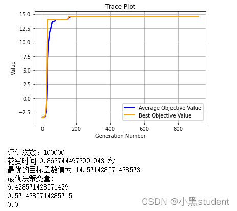
print('评价次数：%s'%(myAlgorithm.evalsNum))
print('花费时间 %s 秒'%(myAlgorithm.passTime))
if BestIndi.sizes != 0:
    print("最优的目标函数值为 %s" % BestIndi.ObjV[0][0])
    print("最优决策变量:")
    for i in range(BestIndi.Phen.shape[1]):
        print(BestIndi.Phen[0, i])
else:
    print("未找到解")

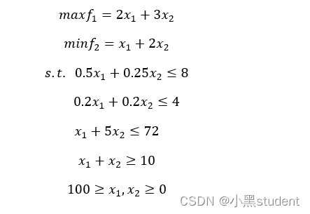
例2 多目标规划

#问题对象
class MyProblem(ea.Problem):
    def __init__(self):
        name = "MOP"
        M = 2
        maxormins = [-1, 1] #-1：第一个函数最大值，1：第二个函数最小值
        Dim = 2
        varTypes = [0] * Dim
        lb = [0, 0]
        ub = [100, 100]
        lbin = [1] * Dim
        ubin = [0] * Dim
        ea.Problem.__init__(self, name, M, maxormins, Dim, varTypes, lb, ub, lbin, ubin)
        
    def aimFunc(self, pop):
        Vars = pop.Phen
        
        x1 = Vars[:, [0]]
        x2 = Vars[:, [1]]
        f1 = 2 * x1 + 3 * x2
        f2 = x1 + 2 * x2
        pop.ObjV = np.hstack([f1, f2])
        pop.CV = np.hstack([ #约束条件全部化成小于等于0的形式
            0.5 * x1 + 0.25 * x2 - 8,
            0.2 * x1 + 0.2 * x2 - 4,
            x1 + 5 * x2 - 72,
            10 - x1 - x2
        ])

problem = MyProblem()

Encoding="RI"
NIND = 200
Field = ea.crtfld(Encoding, problem.varTypes, problem.ranges, problem.borders)
population = ea.Population(Encoding, Field, NIND)

#使用NSGA2解决多目标规划问题
myAlgorithm = ea.moea_NSGA2_templet(problem, population)
myAlgorithm.MAXGEN = 500
myAlgorithm.mutOper.Pm = 0.3
myAlgorithm.recOper.XOVR = 0.8
myAlgorithm.logTras = 1
myAlgorithm.verbose = False
myAlgorithm.drawing = 1

[NDSet, population] = myAlgorithm.run()
print("用时: %s"%(myAlgorithm.passTime))
print("非支配个体数: %d"%NDSet.sizes) if NDSet.sizes != 0 else print("没有可行解")
if myAlgorithm.log is not None and NDSet.sizes != 0:
    print("HV: ", myAlgorithm.log["hv"][-1])
    print("Spacing: ", myAlgorithm.log["spacing"][-1])
    
if NDSet.sizes != 0:
    print("最优决策变量:")
    for i in range (NDSet.Phen.shape[1]):
        print(f"x{i}: {NDSet.Phen[0, i]}")
metricName = [["hv"]]
metric = np.array([myAlgorithm.log[metricName[i][0]] for i in range(len(metricName))]).T
ea.trcplot(metric, labels=metricName, titles=metricName)

可以求出决策变量的值为多少，再代入两个函数式中。但每次运行结果不同，每次带入计算， 选择最优的那一个解即可

参考资料

python遗传算法之单/多目标规划问题