决策树对wine数据集进行分类

对红酒品种进行分类。

Wine葡萄酒数据集是来自UCI上面的公开数据集，这些数据是对意大利同一地区种植的葡萄酒进行化学分析的结果，这些葡萄酒来自三个不同的品种。该分析确定了三种葡萄酒中每种葡萄酒中含有的13种成分的数量。

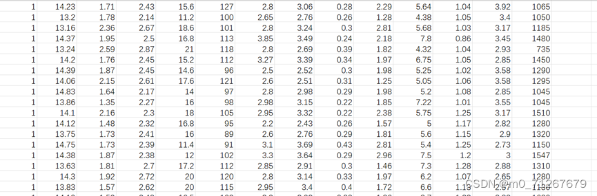
在wine数据集中，这些数据包括了三种酒中13种不同成分的数量。文件中，每行代表一种酒的样本，共有178个样本；一共有14列，其中，第一个属性是类标识符，分别是1/2/3来表示，代表葡萄酒的三个分类。后面的13列为每个样本的对应属性的样本值。剩余的13个属性是，酒精、苹果酸、灰、灰分的碱度、镁、总酚、黄酮类化合物、非黄烷类酚类、原花色素、颜色强度、色调、稀释葡萄酒的OD280/OD315、脯氨酸。其中第1类有59个样本，第2类有71个样本，第3类有48个样本。

# 引入数据

from sklearn import datasets

import numpy as np

from sklearn.preprocessing import StandardScaler

import pandas as pd

names=['0Alcohol','1Malic acid ','2Ash','3Alcalinity of ash',

         '4Magnesium','5Total phenols','6Flavanoid',

         '7Nonflavanoid phenols','8Proanthocyanins ','9Color intensity ','10Hue ','11OD280/OD315 of diluted wines' ,'12Proline ','13category']

wine=pd.read_csv(r"D:\user\桌面\wine.csv",names=names)

x= wine.iloc[:,1:]

y = wine.iloc[:,0]

#对数据进行归一化，便于更好的训练模型

scaler=StandardScaler()

x_new=scaler.fit_transform(x)

# print(x_new)

#根据线性回归函数提取出与样本标签最相关的两个特征值，选则两个特征便于绘制决策边界图

from sklearn.feature_selection import SelectKBest,f_regression

selector=SelectKBest(f_regression,k=2)

X=selector.fit_transform(x_new,y)

# print(X)

#辨别对红酒的样本标签影响最大的两种特征是哪两种

types=selector.get_support(indices=True).tolist()

for i in range(2):

    types[i]+=1

print(types,wine.columns[types])

# 切分训练数据和测试数据

from sklearn.model_selection import train_test_split

# 30%测试数据，70%训练数据,stratify=y表示训练数据和测试数据具有相同的类别比例

X_train,X_test,y_train,y_test = train_test_split(X,y,test_size=0.3,random_state=1,stratify=y)

kind,count=np.unique(y_train,return_counts=True)

# print(kind,count)

kind_test,count_test=np.unique(y_test,return_counts=True)

# print(kind,count_test)

# 决策树分类器  标准化之后的数据

from sklearn.tree import DecisionTreeClassifier

#利用网格搜索调参数，找到最合适的参数使得模型更精确

from sklearn. model_selection import GridSearchCV

parameters = {'max_depth' : [1,3,5, 7, 9, 11, 13], 'criterion' : ['gini','entropy' ]}

model = DecisionTreeClassifier (random_state=1)

grid_search = GridSearchCV (model, parameters, scoring='accuracy', cv=5)

# 传入训练集数据并开始进行参数调优

grid_search.fit (X_train, y_train)

#输出参数的最优值

best_depth=grid_search.best_params_

print(best_depth)

tree=DecisionTreeClassifier(criterion='gini',max_depth= 3,random_state=1)

tree.fit(X_train,y_train)

accuracy=tree.score(X_test, y_test)

print("模型准确度为",accuracy)

print(tree)

#绘制决策树

from sklearn.tree import plot_tree

plt.figure(figsize=(15,9))

plot_tree(tree,filled=True,feature_names=['7Nonflavanoid phenols', '12Proline '], class_names=['1','2','3'])

plt.show()

# 画出决策边界图(只有在2个特征才能画出来)

import matplotlib.pyplot as plt

from matplotlib.colors import ListedColormap

def plot_decision_region(X, y, classifier, resolution=0.02):

    markers = ['s', 'x', 'o']

    colors = ['red', 'blue', 'lightgreen']

    # 背景色

    #np.unique(y)y的种类有三种

    #ListedColormap函数用于颜色转化，构建一个对象存放colors

    cmap = ListedColormap(colors[:len(np.unique(y))])

    # 这里+1  -1的操作我理解为防止样本落在图的边缘

    x1_min, x1_max = X[:, 0].min() - 1, X[:, 0].max() + 1

    # print(x1_min, x1_max)



    x2_min, x2_max = X[:, 1].min() - 1, X[:, 1].max() + 1

    # print(x2_min, x2_max)



    # 生成网格点坐标矩阵

    #np.arange(x1_min, x1_max, resolution),在第一列特征值的最大值和最小值之间以0.01为步长生成数组

    #np.meshgrid(a, b) 函数会返回 b.shape() 行 ，a.shape() 列的二维数组。

    xx1, xx2 = np.meshgrid(np.arange(x1_min, x1_max, resolution),

                           np.arange(x2_min, x2_max, resolution))

    #x.ravel函数是将其二维数组铺展开，降成为一维数组

    #c_函数将两个二维数组左右拼接在一起

    # print(np.c_[xx1.ravel(), xx2.ravel()])

    #Z是指绘制鞭策轮廓对应的值，也就是和三种预测类别

    Z = classifier.predict(np.c_[xx1.ravel(), xx2.ravel()])

    np.set_printoptions(threshold=np.inf)#将省略信息可以被print出来

    #reshape函数将数组转化为与特征值大小相同的行数和列数的数组，这是因为在绘制轮廓等高线的时候，针对多维数据必须将他们的形状保持一致

    Z = Z.reshape(xx1.shape)

    # print(xx1,xx2)

    # print(Z)

    # 绘制轮廓等高线  alpha参数为透明度

    plt.contourf(xx1, xx2, Z, alpha=0.3, cmap=cmap)

    #设置x轴y轴的显示范围

    plt.xlim(xx1.min(), xx1.max())

    plt.ylim(xx2.min(), xx2.max())

    # plot class samples

    for i in np.unique(y):

        # 这是针对数组的切片操作：X[y==0,0]是用来进行切片，y==0在鸢尾花中的数据集选择出类别为0对应的特征值

        plt.scatter(x=X[y == i, 0],

                    y=X[y == i, 1],

                    alpha=0.8,

                    c=colors[i-1],

                    marker=markers[i-1],

                    label=i,

                    edgecolors='black')

plot_decision_region(X_train,y_train,classifier=tree,resolution=0.01)

plt.xlabel('7Nonflavanoid phenols')

plt.ylabel('12Proline')

plt.legend(loc='upper left')

plt.show()