ggstatsplot | 一个满足你日常统计需求的高颜值R包（二）

🤩 ggstatsplot | 一个满足你日常统计需求的高颜值R包（二）

1. 加载需要的R包

rm(list=ls())
library(ggstatsplot)
library(ggplot2)

2. 用到的数据

dat <- bugs_long

3. 重复测量数据的比较

一个组别如果分别在多个时间点被采集数据，这种情况就归属于重复测量设计，就不能采用ggbetweenstats了，因为已经违反了独立性的原则。

这里介绍另一个函数，ggwithinstats

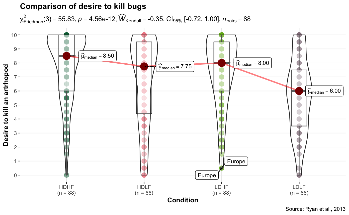
3.1 初步绘制

默认是boxviolinplot~

ggwithinstats(
  data = dat,
  x = condition,
  y = desire
)

Note! 此处x轴应为不同时间点，红色线条注明它们之间为配对样本。

---

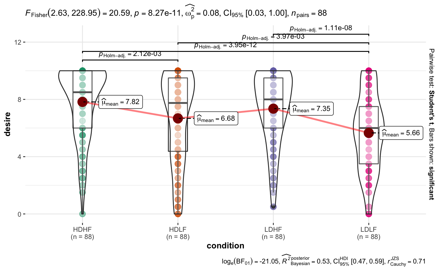
3.2 修改细节

type 为可选统计类型包括
✅ "p" → parametric
✅ "np" → non-parametric
✅ "r" → robust
✅ "bf" → Bayesian

ggwithinstats(
  data = dat,
  x = condition,
  y = desire,
  type = "nonparametric", ## 统计方法
  xlab = "Condition", ## x轴的label
  ylab = "Desire to kill an artrhopod", ## y轴的label
  effsize.type = "biased", ## 效应值类型
  sphericity.correction = FALSE, ## 不显示校正后的DFS和P值
  pairwise.comparisons = TRUE, ## 显示配对比较
  outlier.tagging = TRUE, ## 是否标记outlier
  outlier.coef = 1.5, ##  Tukey's rule的系数
  outlier.label = region, ## 标记outlier的label
  outlier.label.color = "red", ## 标记outlier的label的颜色
  mean.plotting = TRUE, ## 是否显示均值
  mean.color = "darkblue", ## 均值的颜色
  package = "yarrr", ## 颜色所取的包
  palette = "info2", ## 所取的调色板
  title = "Comparison of desire to kill bugs",
  caption = "Source: Ryan et al., 2013"
) + ## 再改一下y轴limit
  ggplot2::scale_y_continuous(
    limits = c(0, 10),
    breaks = seq(from = 0, to = 10, by = 1)
  )

---

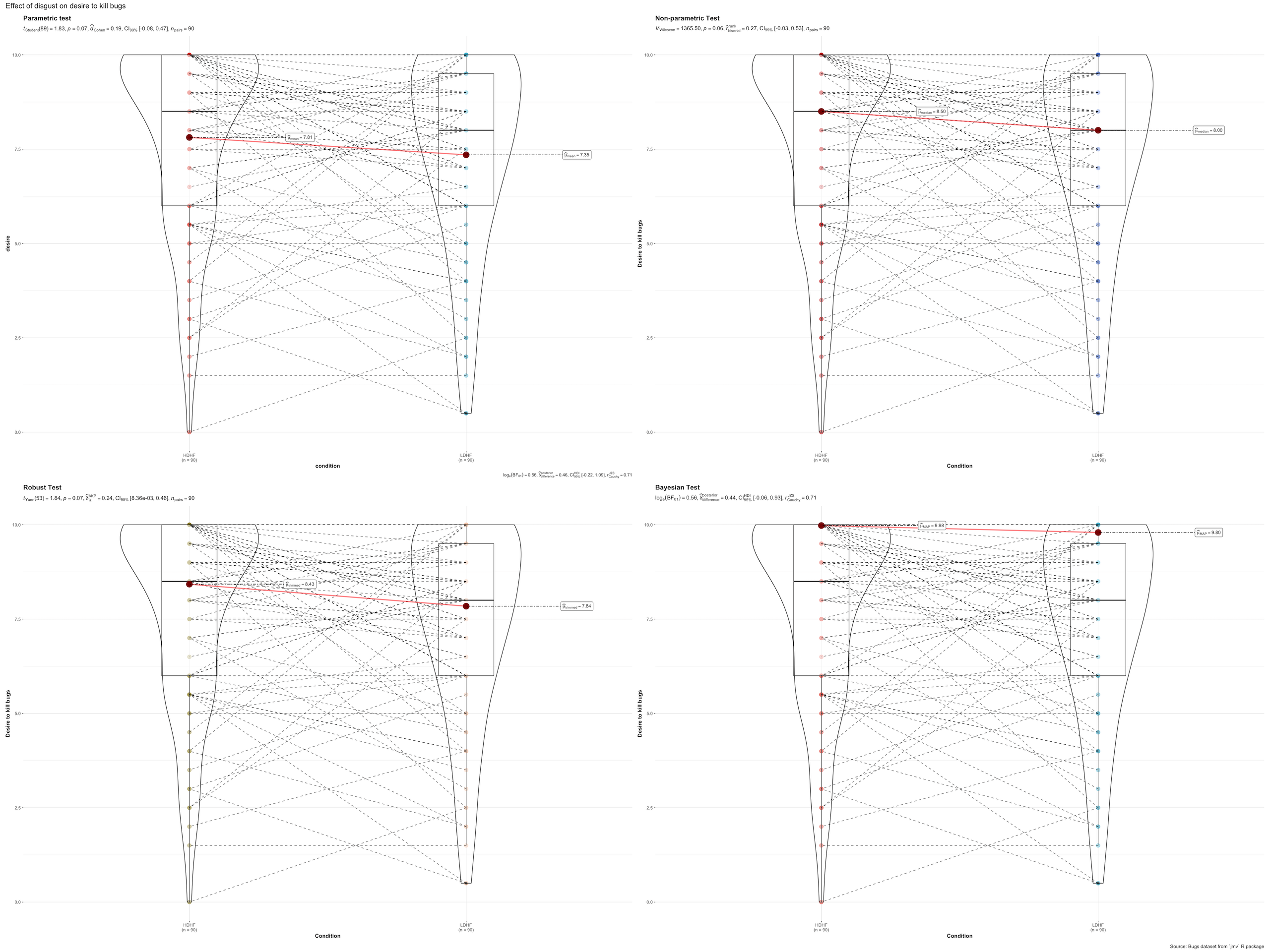
3.3 用四种不同统计方法并拼图

只需要修改type参数，再利用combined_plots即可

## 由于数据量较大，在此只选择condition为LDHF何HDHF进行演示
df_disgust <- dplyr::filter(dat, condition %in% c("LDHF", "HDHF"))

开始统计绘图

## parametric t-test
p1 <- ggwithinstats(
  data = df_disgust,
  x = condition,
  y = desire,
  type = "p",
  effsize.type = "d",
  conf.level = 0.99,
  title = "Parametric test",
  package = "ggsci",
  palette = "nrc_npg"
)

## Mann-Whitney U test (nonparametric test)
p2 <- ggwithinstats(
  data = df_disgust,
  x = condition,
  y = desire,
  xlab = "Condition",
  ylab = "Desire to kill bugs",
  type = "np",
  conf.level = 0.99,
  title = "Non-parametric Test",
  package = "ggsci",
  palette = "uniform_startrek"
)

## robust t-test
p3 <- ggwithinstats(
  data = df_disgust,
  x = condition,
  y = desire,
  xlab = "Condition",
  ylab = "Desire to kill bugs",
  type = "r",
  conf.level = 0.99,
  title = "Robust Test",
  package = "wesanderson",
  palette = "Royal2"
)

## Bayes Factor for parametric t-test
p4 <- ggwithinstats(
  data = df_disgust,
  x = condition,
  y = desire,
  xlab = "Condition",
  ylab = "Desire to kill bugs",
  type = "bayes",
  title = "Bayesian Test",
  package = "ggsci",
  palette = "nrc_npg"
)

## combine_plots函数绘制在一张图上
combine_plots(
  plotlist = list(p1, p2, p3, p4),
  plotgrid.args = list(nrow = 2),
  annotation.args = list(
    title = "Effect of disgust on desire to kill bugs ",
    caption = "Source: Bugs dataset from `jmv` R package"
  )
)

---

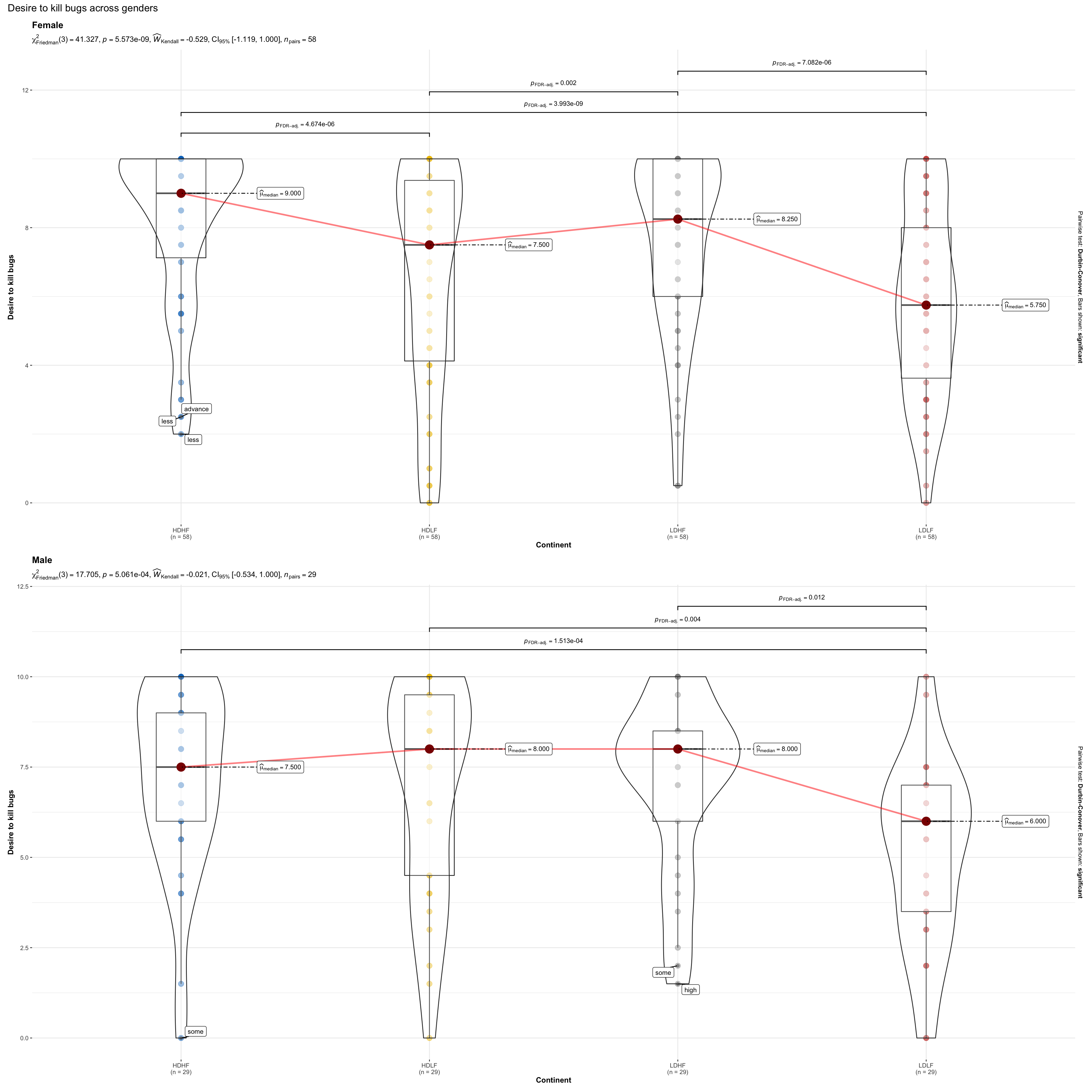
4. 复杂分组重复测量比较

比较不同gender的condition各组的desire

grouped_ggwithinstats(
  data = dat,
  x = condition,
  y = desire,
  grouping.var = gender,
  xlab = "Continent",
  ylab = "Desire to kill bugs",
  type = "nonparametric", 
  pairwise.display = "significant",
  p.adjust.method = "BH", 
  package = "ggsci",
  palette = "default_jco",
  outlier.tagging = TRUE,
  outlier.label = education,
  k = 3,
  ## arguments relevant for combine_plots
  annotation.args = list(title = "Desire to kill bugs across genders"),
  plotgrid.args = list(ncol = 1)
)

---

5. 一次性应用不同分析方法

和ggbetweens联合purr包相似，我们也可以用同样的方法进行批量绘制

这里我们使用ez包里的ANT数据作为示例数据

library(ez)
data("ANT") 

---

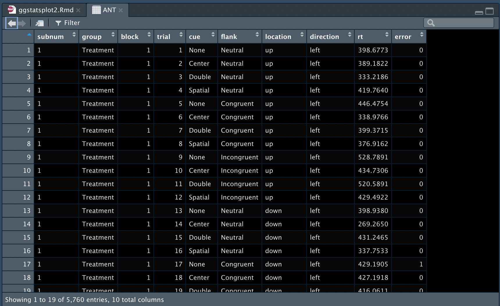
首先进行数据处理

## 转为list格式
cue_list <- ANT %>% 
  split(f = .$cue, drop = TRUE)

## 查看list参数
# length(cue_list)
# names(cue_list)

## 用`pmap`函数进行批量绘制
plot_list <- purrr::pmap(
  .l = list(
    data = cue_list,
    x = "flank",
    y = "rt",
    outlier.tagging = TRUE,
    outlier.label = "group",
    outlier.coef = list(2, 2, 2.5, 3),
    outlier.label.args = list(
      list(size = 3, color = "#56B4E9"),
      list(size = 2.5, color = "#009E73"),
      list(size = 4, color = "#F0E442"),
      list(size = 2, color = "red")
    ),
    xlab = "Flank",
    ylab = "Response time",
    title = list(
      "Cue: None",
      "Cue: Center",
      "Cue: Double",
      "Cue: Spatial"
    ),
    type = list("p", "r", "bf", "np"),
    pairwise.display = list("ns", "s", "ns", "all"),
    p.adjust.method = list("fdr", "hommel", "bonferroni", "BH"),
    conf.level = list(0.99, 0.99, 0.95, 0.90),
    k = list(3, 2, 2, 3),
    effsize.type = list(
      "omega",
      "eta",
      "partial_omega",
      "partial_eta"
    ),
    package = list("ggsci", "palettetown", "palettetown", "wesanderson"),
    palette = list("lanonc_lancet", "venomoth", "blastoise", "GrandBudapest1"),
    ggtheme = list(
      ggplot2::theme_linedraw(),
      hrbrthemes::theme_ft_rc(),
      ggthemes::theme_solarized(),
      ggthemes::theme_gdocs()
    )
  ),
  .f = ggwithinstats
)

---

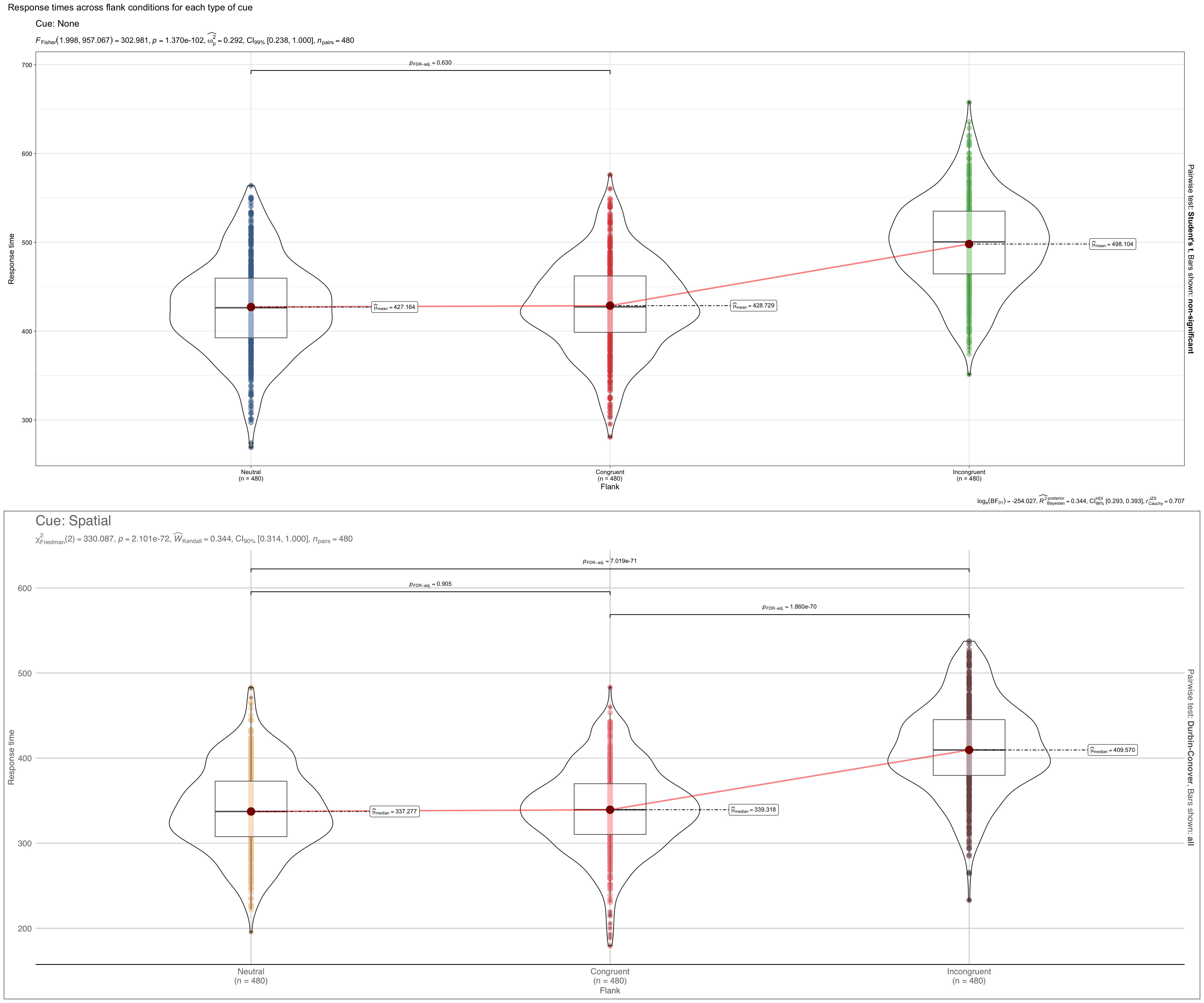
最后利用combine_plots函数进行可视化

# 图太大，就只做第一个和第四个的可视化
combine_plots(
  plotlist = plot_list[c(1,4)],
  annotation.args = list(title = "Response times across flank conditions for each type of cue"),
  plotgrid.args = list(ncol = 1)
)

---

最后祝大家早日不卷!~

---

点个在看吧各位~ ✐.ɴɪᴄᴇ ᴅᴀʏ 〰