Slingshot | 细胞分化轨迹的这样做比较简单哦！~（一）

最新推荐文章于 2024-07-10 23:54:36 发布

生信漫卷

最新推荐文章于 2024-07-10 23:54:36 发布

阅读量569

点赞数

文章标签：后端

本文链接：https://blog.csdn.net/m0_72224305/article/details/132384923

版权

1写在前面

今天是医师节，祝各位医护节日快乐，夜班平安，病历全是甲级，没有错误。🥰

不知道各位医师节的福利是什么！？😂

我们医院是搞了义诊活动，哈哈哈哈哈哈哈。🫠

这么好的节日，以后尽量别搞了。😭

2用到的包

rm(list = ls())
library(slingshot)
library(tidyverse)
library(uwot)	
library(mclust)
library(RColorBrewer)
library(grDevices)

3示例数据

means <- rbind(
    matrix(rep(rep(c(0.1,0.5,1,2,3), each = 300),100),
        ncol = 300, byrow = T),
    matrix(rep(exp(atan( ((300:1)-200)/50 )),50), ncol = 300, byrow = T),
    matrix(rep(exp(atan( ((300:1)-100)/50 )),50), ncol = 300, byrow = T),
    matrix(rep(exp(atan( ((1:300)-100)/50 )),50), ncol = 300, byrow = T),
    matrix(rep(exp(atan( ((1:300)-200)/50 )),50), ncol = 300, byrow = T),
    matrix(rep(exp(atan( c((1:100)/33, rep(3,100), (100:1)/33) )),50), 
        ncol = 300, byrow = TRUE)
)

counts <- apply(means,2,function(cell_means){
    total <- rnbinom(1, mu = 7500, size = 4)
    rmultinom(1, total, cell_means)
})
rownames(counts) <- paste0('G',1:750)
colnames(counts) <- paste0('c',1:300)
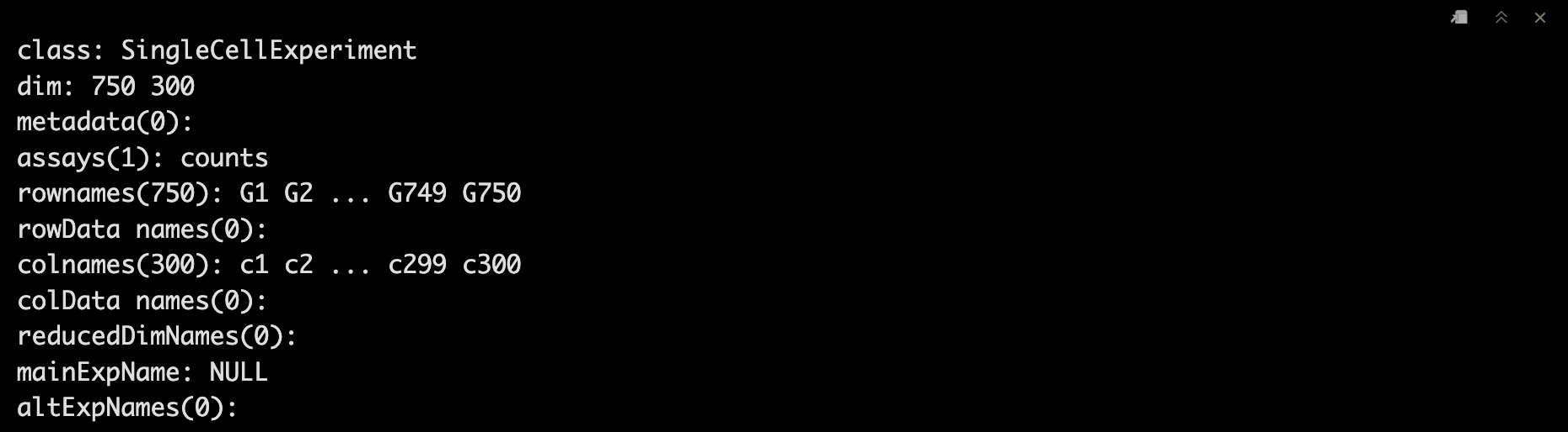
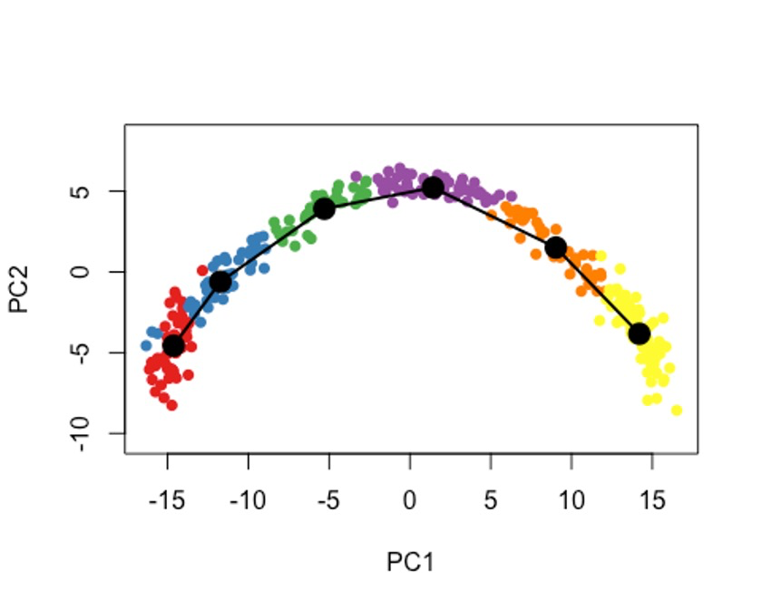
sce <- SingleCellExperiment(assays = List(counts = counts))
sce

4基因过滤

这里我们把cluster size设置为≥10，count设置为≥3，以这个条件进行过滤，筛选过一些低表达的。😏

geneFilter <- apply(assays(sce)$counts,1,function(x){
    sum(x >= 3) >= 10
})
sce <- sce[geneFilter, ]

5Normalization

接着我们做一下Normalization，去除一些技术因素或者生物学因素上的影响，比如batch,sequencing depth, cell cycle等等。🥰

FQnorm <- function(counts){
    rk <- apply(counts,2,rank,ties.method='min')
    counts.sort <- apply(counts,2,sort)
    refdist <- apply(counts.sort,1,median)
    norm <- apply(rk,2,function(r){ refdist[r] })
    rownames(norm) <- rownames(counts)
    return(norm)
}
assays(sce)$norm <- FQnorm(assays(sce)$counts)

6降维

这里我们用2种方法来试试，PCA和UMAP。😂

6.1 方法一

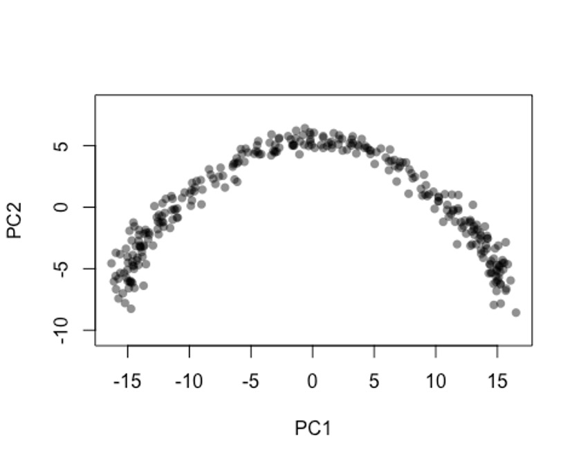
在做PCA的时候，大家尽量不要对基因的表达量做scale，这样的结果会更准一些。🤐

pca <- prcomp(t(log1p(assays(sce)$norm)), scale. = F)
rd1 <- pca$x[,1:2]

plot(rd1, col = rgb(0,0,0,.5), pch=16, asp = 1)

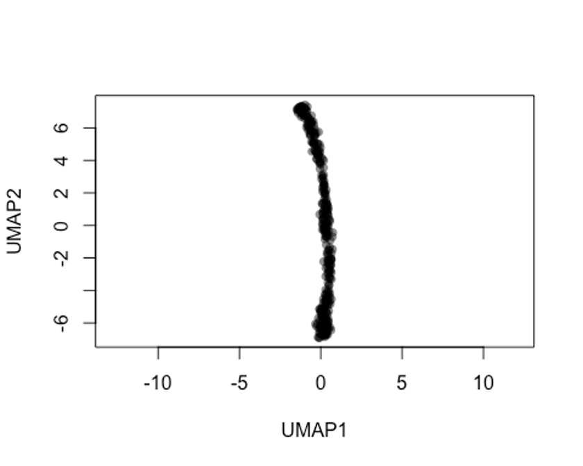
6.2 方法二

rd2 <- uwot::umap(t(log1p(assays(sce)$norm)))
colnames(rd2) <- c('UMAP1', 'UMAP2')

plot(rd2, col = rgb(0,0,0,.5), pch=16, asp = 1)

然后我们把结果存在到之前的SingleCellExperiment文件sce里吧。😜

reducedDims(sce) <- SimpleList(PCA = rd1, UMAP = rd2)

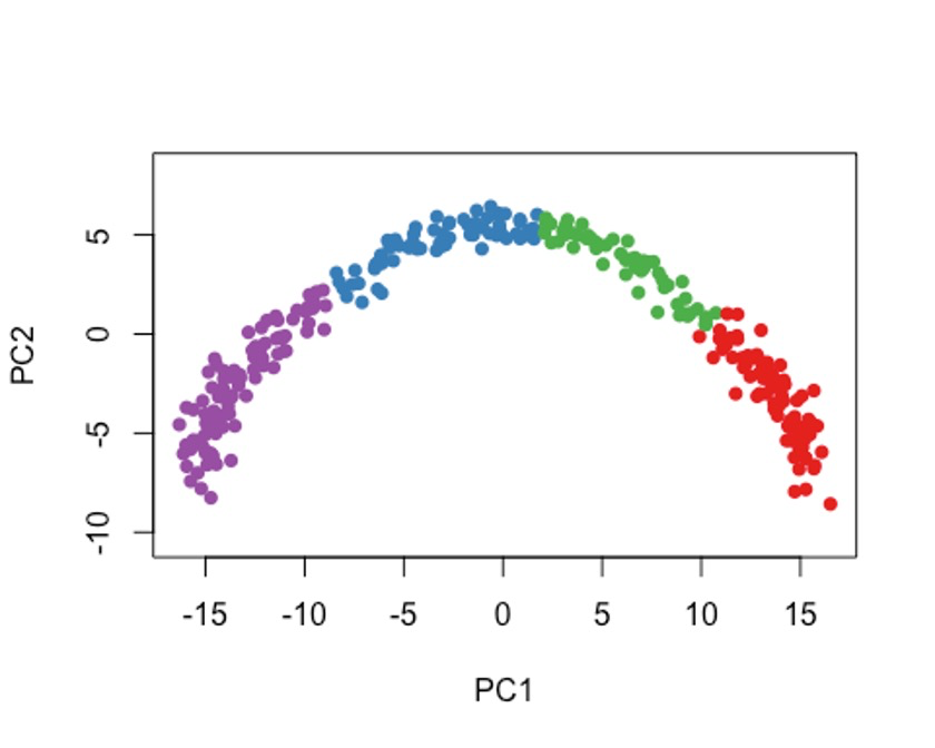
7细胞聚类

这里我们也提供2种方法吧，Gaussian mixture modeling和k-means。🥳

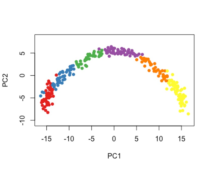
7.1 方法一

cl1 <- Mclust(rd1)$classification
colData(sce)$GMM <- cl1

plot(rd1, col = brewer.pal(9,"Set1")[cl1], pch=16, asp = 1)

7.2 方法二

cl2 <- kmeans(rd1, centers = 4)$cluster
colData(sce)$kmeans <- cl2

plot(rd1, col = brewer.pal(9,"Set1")[cl2], pch=16, asp = 1)

8slingshot进行Pseudotime分析

sce <- slingshot(sce, clusterLabels = 'GMM', reducedDim = 'PCA')

summary(sce$slingPseudotime_1)

colData(sce)$slingshot

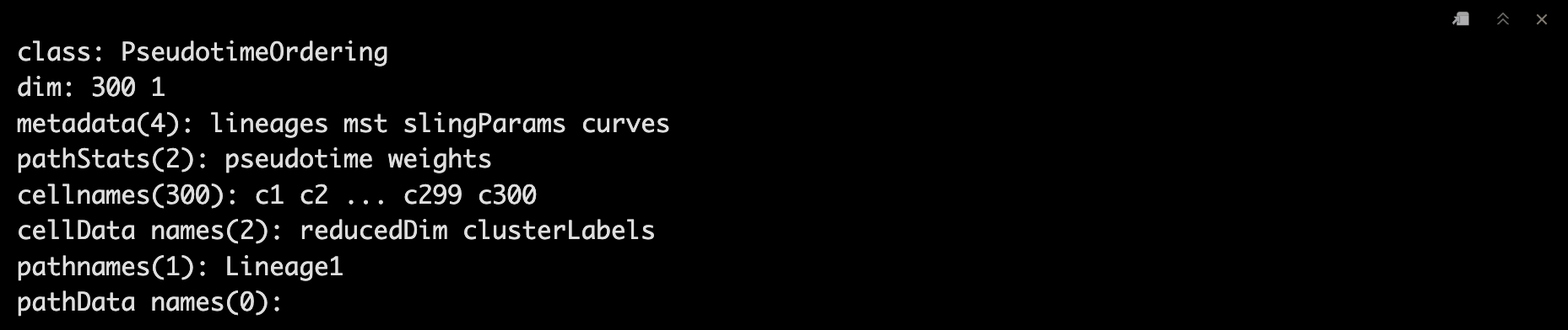
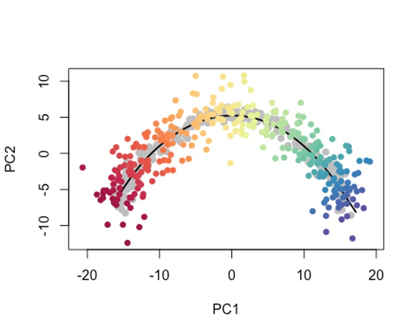
single-trajectory 🤩

colors <- colorRampPalette(brewer.pal(11,'Spectral')[-6])(100)
plotcol <- colors[cut(sce$slingPseudotime_1, breaks=100)]

plot(reducedDims(sce)$PCA, col = plotcol, pch=16, asp = 1)
lines(SlingshotDataSet(sce), lwd=2, col='black')

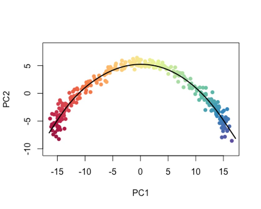
当然，你也可以把type设置为lineages，模拟以cluster为单位的变化过程。🤓

plot(reducedDims(sce)$PCA, col = brewer.pal(9,'Set1')[sce$GMM], pch=16, asp = 1)
lines(SlingshotDataSet(sce), lwd=2, type = 'lineages', col = 'black')

9大数据的处理

示例数据都比较小，但实际你测完的数据可能会非常大。😜

这个时候我们要加上一个参数，approx_points，默认是150，一般选择100-200。🫠

如果你把approx_points设置为False，会获得尽可能多的点，和data中的细胞数有一定的关系。😭

sce5 <- slingshot(sce, clusterLabels = 'GMM', reducedDim = 'PCA',
                   approx_points = 150)

colors <- colorRampPalette(brewer.pal(11,'Spectral')[-6])(100)
plotcol <- colors[cut(sce5$slingPseudotime_1, breaks=100)]

plot(reducedDims(sce5)$PCA, col = plotcol, pch=16, asp = 1)
lines(SlingshotDataSet(sce5), lwd=2, col='black')

10将细胞投射到现有轨迹上

可能有时候，我们只想使用细胞的一个子集或者新的data来确定轨迹，我们都需要一种方法来确定新细胞沿着先前构建的轨迹的位置。🤓

这个时候我们可以用predict函数，

pto <- sce$slingshot

newPCA <- reducedDim(sce, 'PCA') + rnorm(2*ncol(sce), sd = 2)

newPTO <- slingshot::predict(pto, newPCA)

原细胞轨迹为灰色哦。🫠

newplotcol <- colors[cut(slingPseudotime(newPTO)[,1], breaks=100)]
plot(reducedDims(sce)$PCA, col = 'grey', bg = 'grey', pch=21, asp = 1,
     xlim = range(newPCA[,1]), ylim = range(newPCA[,2]))
lines(SlingshotDataSet(sce), lwd=2, col = 'black')
points(slingReducedDim(newPTO), col = newplotcol, pch = 16)

最后祝大家早日不卷!~

点个在看吧各位~ ✐.ɴɪᴄᴇ ᴅᴀʏ 〰

本文由 mdnice 多平台发布