带硬约束的物理信息神经网络（PINN with Hard Constraint）示例及代码

目录

0.摘要

1.问题描述

2.带硬约束的物理信息神经网络

3.参数设置

4.结果展示

5.完整代码

6.总结

---

0.摘要

        本文以一个案例介绍了带硬约束的物理信息神经网络的原理及实现步骤。

1.问题描述

        考虑下面的二阶常微分方程。定义域为[0,1]。

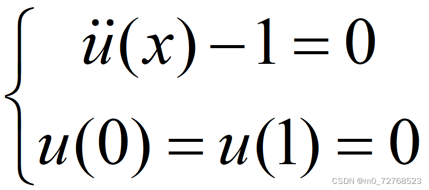
2.带硬约束的物理信息神经网络

        常规的PINN解决这个问题需要同时考虑方程项损失和边界条件项损失，由此带来各项损失权重调整等问题。考虑将边界条件构造进神经网络中，使得网络输出自动满足边界条件，即带硬约束的物理信息神经网络。

        针对本文问题实际，将网络输出经过映射后，自动满足边界条件，可以只考虑方程项损失。代码如下：

    def forward(self, x):
        if torch.is_tensor(x) == False:
            x = torch.from_numpy(x)
        a = x.float()
        for i in range(len(layers)-2):
            z = self.linears[i](a)
            a = self.activation(z)
        a = self.linears[-1](a)
        def transform(x, y):
            return torch.sin(torch.pi*x) * y
        return transform(x, a)

3.参数设置

        本文基于pytorch平台编写代码，神经网络相关参数：网络架构为，学习率为0.0001，激活函数为tanh，优化器为Adam，训练10000轮。

4.结果展示

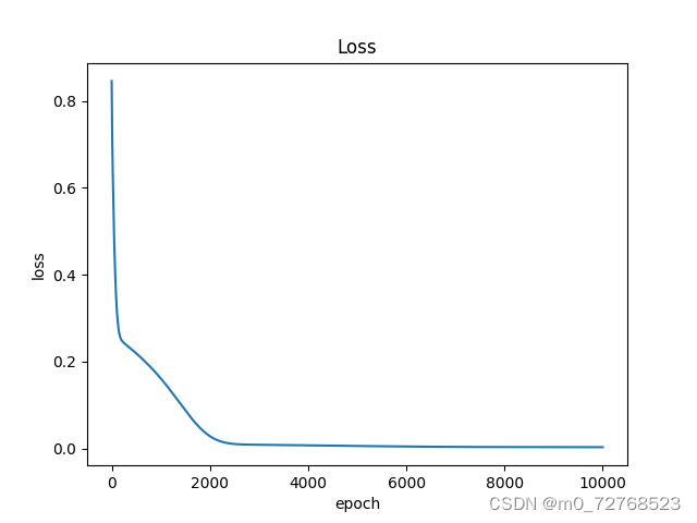
图1 损失下降曲线

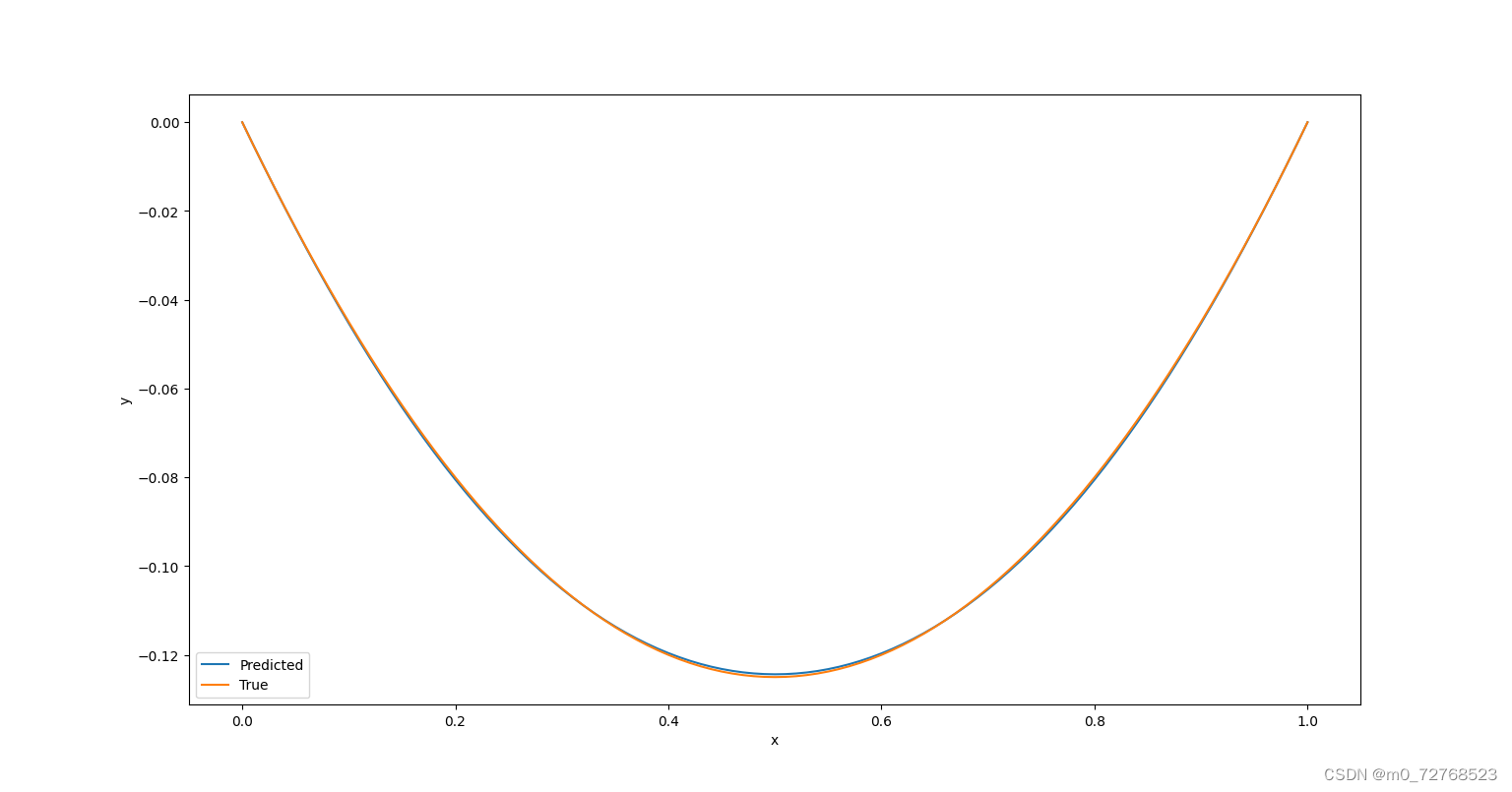
图2 结果图像

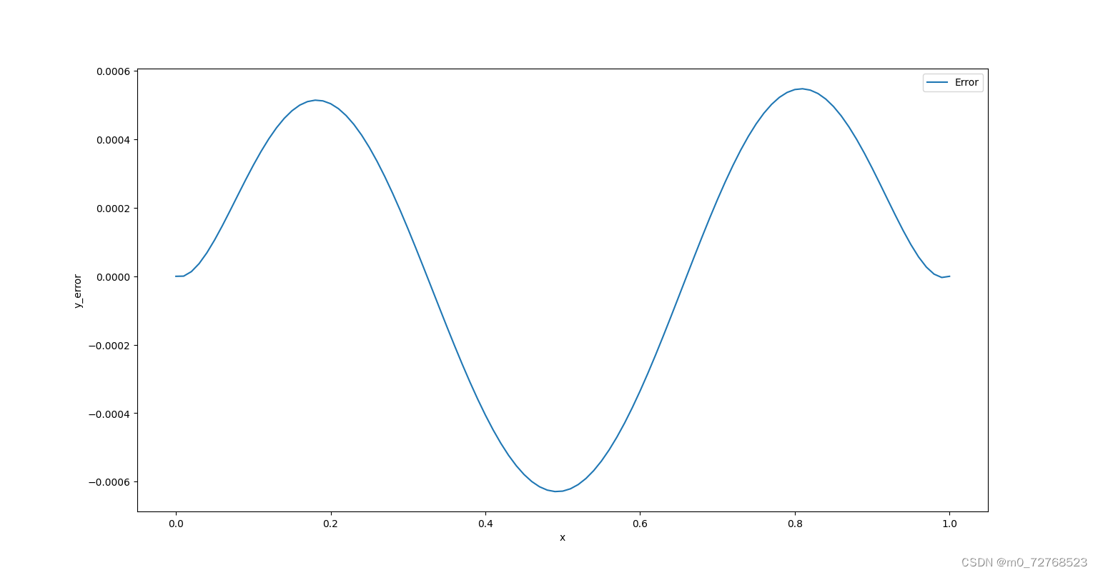图3 误差曲线

        从损失曲线看，网络训练良好，从结果图像及误差曲线看，硬约束的施加使得网络输出自动满足边界条件，避免了繁琐的权重调整，同时也降低了误差。

5.完整代码

import time
import torch
import torch.autograd as autograd
import torch.nn as nn
import numpy as np
import matplotlib.pyplot as plt

torch.set_default_dtype(torch.float)

torch.manual_seed(1234)

np.random.seed(1234)

device = torch.device('cuda' if torch.cuda.is_available() else 'cpu')
print(device)

if device == 'cuda':
    print(torch.cuda.get_device_name())

class FCN(nn.Module):
    def __init__(self, layers):
        super().__init__()
        self.activation = nn.Tanh()
        self.loss_function = nn.MSELoss(reduction='mean')
        self.linears = nn.ModuleList([nn.Linear(layers[i], layers[i+1]) for i in range(len(layers)-1)])
        self.iter = 0

        for i in range(len(layers)-1):
            nn.init.xavier_normal_(self.linears[i].weight.data, gain=1.0)
            nn.init.zeros_(self.linears[i].bias.data)

    def forward(self, x):
        if torch.is_tensor(x) == False:
            x = torch.from_numpy(x)
        a = x.float()
        for i in range(len(layers)-2):
            z = self.linears[i](a)
            a = self.activation(z)
        a = self.linears[-1](a)
        def transform(x, y):    #硬约束施加
            return torch.sin(torch.pi*x) * y
        return transform(x, a)

    def lossPDE(self, x_PDE):
        g = x_PDE.clone()
        g.requires_grad = True
        f = self.forward(g)
        f_x = autograd.grad(f, g, torch.ones_like(g).to(device), retain_graph=True, create_graph=True)[0]
        f_xx = autograd.grad(f_x, g, torch.ones_like(g).to(device), create_graph=True)[0]
        f = f_xx - 1
        return self.loss_function(f, torch.zeros_like(f))

x = torch.linspace(0, 1, 101).reshape(-1,1)
index = torch.randperm(x.size(0))
x = x[index]
x_train = x.float().to(device)

#网络参数设置
steps = 10000
lr = 1e-4
layers = np.array([1, 50, 1])

PINN = FCN(layers)
PINN.to(device)
print(PINN)
params = list(PINN.parameters())
optimizer = torch.optim.Adam(PINN.parameters(), lr=lr, amsgrad=False)
losses = []

start_time = time.time()
for i in range(steps):
    if i == 0:
        print('Start Training')
    loss = PINN.lossPDE(x_train)
    optimizer.zero_grad()
    loss.backward()
    optimizer.step()
    losses.append(loss.item())

    if i%100 == 0:
        print(f'epoch:{i}','loss:',loss.detach().cpu().numpy())

print('Running Time: ', -start_time+time.time())
plt.plot(range(steps), losses)
plt.title('Loss')
plt.xlabel('epoch')
plt.ylabel('loss')
plt.show()

path_state_dict = './model_state_dict.pkl'
net_state_dict = PINN.state_dict()
torch.save(net_state_dict, path_state_dict)

Net_new = FCN(layers).to(device)
path_state_dict = r'D:\Python1\PINN\model_state_dict.pkl'
state_dict_load = torch.load(path_state_dict)
Net_new.load_state_dict(state_dict_load)

x_test = torch.linspace(0, 1, 101).reshape(-1,1).to(device)
y_pred = Net_new(x_test)

x_plot = x_test.detach().cpu().numpy()
y_plot = y_pred.detach().cpu().numpy()
y_true = (-1/2)*x_plot*(1-x_plot)   #理论解

plt.figure(1)
plt.plot(x_plot, y_plot, label='Predicted')
plt.plot(x_plot, y_true, label='True')
plt.xlabel('x')
plt.ylabel('y')
plt.legend()

plt.figure(2)
plt.plot(x_plot,y_true-y_plot,label='Error')
plt.xlabel('x')
plt.ylabel('y_error')
plt.legend()
plt.show()

6.总结

        本文分享了作者在带硬约束的物理信息神经网络方面的一些工作。

        转载请注明出处。