


机器学习 — 模型选择与调优
文章目录
一,交叉验证
1.1 保留交叉验证HoldOut
HoldOut Cross-validation(Train-Test Split)
在这种交叉验证技术中,整个数据集被随机地划分为训练集和验证集。根据经验法则,整个数据集的近70%被用作训练集,其余30%被用作验证集。也就是我们最常使用的,直接划分数据集的方法。
优点:很简单很容易执行。
缺点1:不适用于不平衡的数据集。假设我们有一个不平衡的数据集,有0类和1类。假设80%的数据属于 “0 “类,其余20%的数据属于 “1 “类。这种情况下,训练集的大小为80%,测试数据的大小为数据集的20%。可能发生的情况是,所有80%的 “0 “类数据都在训练集中,而所有 “1 “类数据都在测试集中。因此,我们的模型将不能很好地概括我们的测试数据,因为它之前没有见过 “1 “类的数据。
缺点2:一大块数据被剥夺了训练模型的机会。
在小数据集的情况下,有一部分数据将被保留下来用于测试模型,这些数据可能具有重要的特征,而我们的模型可能会因为没有在这些数据上进行训练而错过。
from sklearn.datasets import load_iris
from sklearn.model_selection import train_test_split

iris = load_iris()
X = iris.data
y = iris.target

#保留交叉验证HoldOut
X_train,X_test,y_train,y_test = train_test_split(X,y,test_size=0.2,random_state=22)

print(y_test)
[0 2 1 2 1 1 1 2 1 0 2 1 2 2 0 2 1 1 2 1 0 2 0 1 2 0 2 2 2 2]
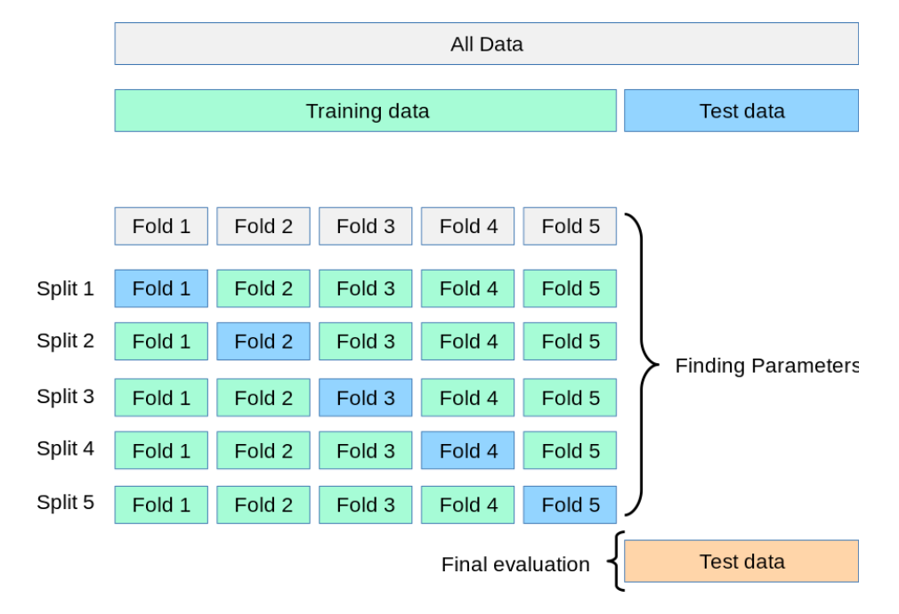
1.2 K-折交叉验证(K-fold)
K-fold Cross Validation,记为K-CV或K-fold)
K-Fold交叉验证技术中,整个数据集被划分为K个大小相同的部分。每个分区被称为 一个”Fold”。所以我们有K个部分,我们称之为K-Fold。一个Fold被用作验证集,其余的K-1个Fold被用作训练集。
该技术重复K次,直到每个Fold都被用作验证集,其余的作为训练集。
模型的最终准确度是通过取k个模型验证数据的平均准确度来计算的。
from sklearn.datasets import load_iris
from sklearn.model_selection import KFold

iris = load_iris()
x = iris.data
y = iris.target

#k-Fold K折交叉验证
kf = KFold(n_splits=5)
index = kf.split(x,y)
for train_index,test_index in index:
    x_train,x_test = x[train_index],x[test_index]
    y_train,y_test = y[train_index],y[test_index]
    print(y_test)

# print(next(index))
[0 0 0 0 0 0 0 0 0 0 0 0 0 0 0 0 0 0 0 0 0 0 0 0 0 0 0 0 0 0]
[0 0 0 0 0 0 0 0 0 0 0 0 0 0 0 0 0 0 0 0 1 1 1 1 1 1 1 1 1 1]
[1 1 1 1 1 1 1 1 1 1 1 1 1 1 1 1 1 1 1 1 1 1 1 1 1 1 1 1 1 1]
[1 1 1 1 1 1 1 1 1 1 2 2 2 2 2 2 2 2 2 2 2 2 2 2 2 2 2 2 2 2]
[2 2 2 2 2 2 2 2 2 2 2 2 2 2 2 2 2 2 2 2 2 2 2 2 2 2 2 2 2 2]
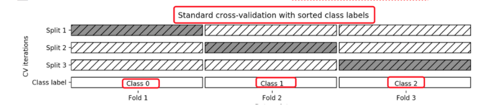
1.3 分层k-折交叉验证Stratified k-fold
Stratified k-fold cross validation,
K-折交叉验证的变种, 分层的意思是说在每一折中都保持着原始数据中各个类别的比例关系,比如说:原始数据有3类,比例为1:2:1,采用3折分层交叉验证,那么划分的3折中,每一折中的数据类别保持着1:2:1的比例,这样的验证结果更加可信。
from sklearn.datasets import load_iris
from sklearn.model_selection import StratifiedKFold

iris = load_iris()
x = iris.data
y = iris.target

#k-Fold K折交叉验证
kf = StratifiedKFold(n_splits=5)
index = kf.split(x,y)
for train_index,test_index in index:
    x_train,x_test = x[train_index],x[test_index]
    y_train,y_test = y[train_index],y[test_index]
    print(y_test)
    break
print(next(index))
[0 0 0 0 0 0 0 0 0 0 1 1 1 1 1 1 1 1 1 1 2 2 2 2 2 2 2 2 2 2]
(array([  0,   1,   2,   3,   4,   5,   6,   7,   8,   9,  20,  21,  22,
        23,  24,  25,  26,  27,  28,  29,  30,  31,  32,  33,  34,  35,
        36,  37,  38,  39,  40,  41,  42,  43,  44,  45,  46,  47,  48,
        49,  50,  51,  52,  53,  54,  55,  56,  57,  58,  59,  70,  71,
        72,  73,  74,  75,  76,  77,  78,  79,  80,  81,  82,  83,  84,
        85,  86,  87,  88,  89,  90,  91,  92,  93,  94,  95,  96,  97,
        98,  99, 100, 101, 102, 103, 104, 105, 106, 107, 108, 109, 120,
       121, 122, 123, 124, 125, 126, 127, 128, 129, 130, 131, 132, 133,
       134, 135, 136, 137, 138, 139, 140, 141, 142, 143, 144, 145, 146,
       147, 148, 149]), array([ 10,  11,  12,  13,  14,  15,  16,  17,  18,  19,  60,  61,  62,
        63,  64,  65,  66,  67,  68,  69, 110, 111, 112, 113, 114, 115,
       116, 117, 118, 119]))
二,超参数搜索
超参数搜索也叫网格搜索(Grid Search)
比如在KNN算法中,k是一个可以人为设置的参数,所以就是一个超参数。网格搜索能自动的帮助我们找到最好的超参数值。
class sklearn.model_selection.GridSearchCV(estimator, param_grid)

说明:
同时进行交叉验证(CV)、和网格搜索(GridSearch),GridSearchCV实际上也是一个估计器(estimator),同时它有几个重要属性:
      best_params_  最佳参数
      best_score_ 在训练集中的准确率
      best_estimator_ 最佳估计器
      cv_results_ 交叉验证过程描述
      best_index_最佳k在列表中的下标
参数:
	estimator: scikit-learn估计器实例
	param_grid:以参数名称(str)作为键,将参数设置列表尝试作为值的字典
		示例: {"n_neighbors": [1, 3, 5, 7, 9, 11]}
    cv: 确定交叉验证切分策略,值为:
        (1)None  默认5折
        (2)integer  设置多少折
        如果估计器是分类器,使用"分层k-折交叉验证(StratifiedKFold)"。在所有其他情况下,使用KFold。
三,鸢尾花数据集示例
from sklearn.neighbors import KNeighborsClassifier
from sklearn.datasets import load_iris
from sklearn.model_selection import train_test_split
from sklearn.model_selection import GridSearchCV
from sklearn.preprocessing import StandardScaler

iris = load_iris()
x,y = load_iris(return_X_y=True)
x_train,x_test,y_train,y_test = train_test_split(x,y,test_size=0.2,random_state=22)

knn_model = KNeighborsClassifier(n_neighbors=5)
model = GridSearchCV(knn_model,param_grid={"n_neighbors":[3,4,5,6,7,8,9,10]},cv=10)

transfer=StandardScaler()
x_train=transfer. fit_transform(x_train)
x_test=transfer.transform(x_test)

model.fit(x_train,y_train)

print("最佳参数:",model.best_params_)
print("最佳结果:",model.best_score_)
print("模型结果:",model.best_estimator_)
y_pred=model.best_estimator_.predict([[1,2,3,4]])
print("预测结果:",y_pred)

print("信息",model.cv_results_)
print("最佳下标",model.best_index_)
最佳参数: {'n_neighbors': 6}
最佳结果: 0.9833333333333332
模型结果: KNeighborsClassifier(n_neighbors=6)
预测结果: [2]
信息 {'mean_fit_time': array([3.00216675e-04, 7.20500946e-05, 6.69097900e-04, 3.50546837e-04,
       5.07640839e-04, 4.11176682e-04, 3.00264359e-04, 2.49981880e-04]), 'std_fit_time': array([0.00045859, 0.00019672, 0.00045004, 0.0004505 , 0.0005081 ,
       0.00050452, 0.00045866, 0.00040276]), 'mean_score_time': array([0.0015717 , 0.0016468 , 0.00132856, 0.00173099, 0.00160072,
       0.00148973, 0.00171149, 0.00175641]), 'std_score_time': array([0.0004462 , 0.00054278, 0.00045266, 0.00043214, 0.00049067,
       0.0004907 , 0.00044354, 0.00033344]), 'param_n_neighbors': masked_array(data=[3, 4, 5, 6, 7, 8, 9, 10],
             mask=[False, False, False, False, False, False, False, False],
       fill_value=999999), 'params': [{'n_neighbors': 3}, {'n_neighbors': 4}, {'n_neighbors': 5}, {'n_neighbors': 6}, {'n_neighbors': 7}, {'n_neighbors': 8}, {'n_neighbors': 9}, {'n_neighbors': 10}], 'split0_test_score': array([1., 1., 1., 1., 1., 1., 1., 1.]), 'split1_test_score': array([0.91666667, 1.        , 1.        , 1.        , 1.        ,
       1.        , 0.91666667, 0.91666667]), 'split2_test_score': array([0.91666667, 1.        , 1.        , 1.        , 1.        ,
       1.        , 1.        , 1.        ]), 'split3_test_score': array([0.91666667, 1.        , 0.91666667, 1.        , 0.91666667,
       0.91666667, 0.91666667, 0.91666667]), 'split4_test_score': array([1.        , 0.91666667, 1.        , 1.        , 1.        ,
       1.        , 1.        , 1.        ]), 'split5_test_score': array([1.        , 0.91666667, 1.        , 1.        , 1.        ,
       1.        , 1.        , 1.        ]), 'split6_test_score': array([0.91666667, 0.91666667, 0.91666667, 0.91666667, 0.91666667,
       0.91666667, 0.91666667, 0.91666667]), 'split7_test_score': array([0.83333333, 0.83333333, 0.91666667, 1.        , 0.91666667,
       0.91666667, 0.91666667, 0.91666667]), 'split8_test_score': array([0.91666667, 0.83333333, 0.91666667, 0.91666667, 0.91666667,
       0.91666667, 0.91666667, 0.91666667]), 'split9_test_score': array([1., 1., 1., 1., 1., 1., 1., 1.]), 'mean_test_score': array([0.94166667, 0.94166667, 0.96666667, 0.98333333, 0.96666667,
       0.96666667, 0.95833333, 0.95833333]), 'std_test_score': array([0.05335937, 0.06508541, 0.04082483, 0.03333333, 0.04082483,
       0.04082483, 0.04166667, 0.04166667]), 'rank_test_score': array([7, 7, 2, 1, 2, 2, 5, 5])}
最佳下标 3
四,现实世界数据集示例
from sklearn.datasets import fetch_20newsgroups
from sklearn.model_selection import train_test_split
from sklearn.feature_extraction.text import TfidfVectorizer
from sklearn.neighbors import KNeighborsClassifier
from sklearn.model_selection import GridSearchCV

news=fetch_20newsgroups(data_home="./src",subset="all")

#  数据集划分
x_train,x_test,y_train,y_test = train_test_split(news.data,news.target,test_size=0.25,random_state=22)

tfidf = TfidfVectorizer()
x_train = tfidf.fit_transform(x_train)
x_test = tfidf.transform(x_test)

# 创建模型
knn_model = KNeighborsClassifier(n_neighbors=5)
# 进行超参数搜索
model = GridSearchCV(knn_model,param_grid={"n_neighbors":[3,4,5,6,7,8,9,10]},cv=10)
model.fit(x_train,y_train)


# 模型评估
score = model.score(x_test,y_test)
print("准确率:",score)
print("最佳参数:",model.best_params_)
print("最佳结果:",model.best_score_)
准确率: 0.7871392190152802
最佳参数: {'n_neighbors': 3}
最佳结果: 0.7871105445394403


 340
340

 被折叠的 条评论
为什么被折叠?
被折叠的 条评论
为什么被折叠?
 到【灌水乐园】发言


