INT202笔记

m0_73819576

已于 2024-05-20 11:07:33 修改

阅读量965

点赞数 21

文章标签：算法数据结构

于 2024-02-28 09:36:10 首次发布

本文链接：https://blog.csdn.net/m0_73819576/article/details/136336668

版权

Lec 1：

1，Algorithms and Data Structures：

A data structure is a systematic way of organizing and accessing data.

An algorithm is a sequence of steps for performing a task in a finite amount of time.

2，Limitations of Experimental Analysis ：

1.Experiments are performed on a limited set of test inputs. 2. Requires all tests to be performed using same hardware and software. 3. Requires implementation and execution of algorithm.

3，Theoretical Analysis Benefits :

1. Can take all possible inputs into account. 2. Can compare efficiency of two (or more) algorithms, independent of hardware/software environment.3. Involves studying high-level descriptions of algorithms (pseudo[1]code).

4，f (n) characterizes the running-time in terms of some measure of the input-size, n.

5, Primitive operations include the following:

• Assigning a value to a variable • Calling a method • Performing an arithmetic operation (for example, adding two numbers) • Comparing two numbers • Indexing into an array • Following an object reference • Returning from a method.

6, Worst-case complexity

refers to running time as the maximum taken over all inputs of the same size.

7, Counting Primitive Operations(不考)

8， Recursive Algorithms

calling itself to solve sub-problems of a smaller size.

require a base case

eg: Algorithm: fibonacci numbers Input: upper limit Nmax Int f(int Nmax) { f1 ← 1; f2 ←1; for n←3:(Nmax-2){ fn← f2 + f1; f1 ← f2; f2 ← fn; return fn; }}

9, Asymptotic notation

Asymptotic notation allows characterization of the main factors affecting running time.

estimates the number of primitive operations.

10, Growth rate

In a log -log chart, the slope of the line corresponds to the growth rate of the function.

The growth rate is not affected by constant factors or lower-order terms.

11, “Big-Oh” Notation

“Big-Oh” notation is probably the most commonly used form of asymptotic notation.

g(n)是f(n)的增长率上限

Given two positive functions f (n) and g(n) (defined on the nonnegative integers), we say f (n) is O(g(n)), written f (n) ∈O(g(n)), if there are constants c and n0 such that:

f (n) ≤ c ·g(n) for all n ≥ n0

eg :Example: 2n + 10 is O(n)---> c = 3 and 𝒏𝟎= 10(默认c > 0 and 𝒏𝟎≥ 1)

eg :If f(n) is a polynomial of degree d, then f(n) is O(𝑛的𝑑次方)

12， Ω(n) and Θ(n) notation

f (n) is Ω(g(n)) (big-Omega) if there are real constants c and n0 such that: f (n) ≥ cg(n) for all n ≥ n0. （f大于等于g）

f (n) is Θ(g(n)) (Theta) if f (n) is Ω(g(n)) and f (n) is also O(g(n)). （f刚好等于g，用f既是O(g(n))也是Ω(g(n))证明）

13, Space Complexity

Space complexity is a measure of the amount of working storage an algorithm needs.

eg : int sum(int x, int y, int z) { int r = x + y + z; return r; }

requires 3 units of space for the parameters and 1 for the local variable, and this never changes, so this is O(1).

Lec 2 data structure:

算法所需和数据类型决定了使用的数据结构

1, Stack：

1.1 A stack is a Last-In, First-Out (LIFO) data structure.

未满前随意插入,可直接访问最后插入。

1.2 A stack is an Abstract Data Type ：

push(Obj)：推入栈顶

pop（）：栈顶移除并返回obj，空则出错

initialize() : initialize a stack

isEmpty() : returns a true if stack is empty, false otherwise.

isFull() : returns a true if stack is full, false otherwise.

1.3 pop push method

pop()先检查 isEmpty（），非空则令 obj =栈顶元素，栈顶= null，return obj

push（obj）先检查 isFull（），未满则索引加一，栈顶赋值

1.4 application：

1.4.1 Reversing an Array ：Push the values from the array onto the stack. Pop the items off the stack into the array.

1.4.2 Reverse Polish notation ：In postfix notation the operands（数字） precede the arithmetic operations （运算符）, e.g. x y +, x y z + ∗ or x y + z ∗. When you encounter an operator, it applies to the previous two operands in the list, in that order.

eg: x y z * + ==> x (y *z) + ==> x + (y*z)

在栈中遇到数字就push入栈，遇到运算符则先pop出栈顶两个数字，运算并返回一个结果到栈顶，直到栈中剩下最终结果。省去了括号，但是注意不要混淆减号和负数。

1.4.3 找出口就是标记老鼠现在点位，并将四周为0的坐标push到栈中，没有则失败，成功则pop出栈顶坐标使它成为现在点位，最终找到出口坐标。关联不大，只记得pop和push用法就好

2, Queue：

2.1 A queue is a First-In, First-Out (FIFO) data structure,

Like queues you’re used to in the real world. ==>从队列后面插入，从队列前移除

2.2 Queue is also ADT. :

enqueue(Obj): inserts object Object the rear of the queue.

dequeue(): 队列前移除并返回，空则出错

size(): Return the number of objects in the queue.

isEmpty(): Returns true if queue is empty, and false otherwise.

isFull(): Returns true if queue is full, and false otherwise. •

front(): 返回队列前的obj，不删除！空则出错

2.3 head and tail

head 指向队列第一个obj，tail是队列最后一个obj的后面的索引。

2.4 Queue and Multiprogramming：

Multiprogramming achieves a limited form of parallelism. ► Allows multiple tasks or threads to be run at the same time.

实现：使用循环协议round robin protocol为线程分配cpu时间，队列前的线程被分配cpu时间，结束后自动替换到队列末尾，以此循环。

3, List :

3.1 A list is a collection of items, with each item being stored in a node which contains a data field and a pointer to the next element in a list. Data can be inserted anywhere in the list by inserting a new node into the list and reassigning pointers. 简单来说就是每个点有数据和指向下一个点的指针，通过重新分配指针可以随意插入。

3.2 Referring methods：

first(): Return position of first element; error occurs if list S is empty.

last(): Return the position of the last element; error occurs if list S is empty.

isFirst(p): Return true if element p is first item in list, false otherwise.

isLast(p): Return true is element p is last element in list, false otherwise.

before(p): Return the position of the element in S preceding the one at position p; error if p is first element.

after(p): Return the position of the element in S following the one at position p; error if p is last element.

3.3 Update methods：

replaceElement(p,e): p - position, e - element.将新元素 e 插入到位置 p

swapElements(p,q): p,q - positions.

insertFirst(e): e - element.

insertLast(e): e - element.

insertBefore(p,e): p - position, e - element.将新元素 e 插入到位置 p 的前面

insertAfter(p,e): p - position, e - element.将新元素 e 插入到位置 p 的后面

remove(p): p - position.

3.4 单链和双链列表

单链列表A node in a singly-linked list stores a next link pointing to next element in list (null if element is last element).

双链列表A node in a doubly-linked list stores two links: a next link, pointing to the next element in list, and a prev link, pointing to the previous element in the list.

3.5 双链列表（注：指针指的都是节点内的元素）

3.5.1 插入 insertAfter(p,e)：

①v.element = e ② v.pre = p ③ v.next = p.next ④ (p.next).pre = v ⑤ p.next = v

3.5.2 删除 remove(p) ：

①t = p.element （返回删除的临时变量） ② (p.prev).next = p.next ③ (p.next).prev = p.prev ④ p.prev = null ⑤ p.next = null ⑥ return t

4, Rooted Trees:

4.1 A rooted tree, T, is a set of nodes which store elements in a parent-child relationship.

4.2 If node u is the parent of node v, then v is a child of u.

Two nodes that are children ofthe same parent are called siblings.

A node is a leaf (external) if it has no children and internal otherwise.

A tree is ordered if there is a linear ordering defined for the children of each internal node.

4.3 Binary Trees : 如果每个节点最多有两个子节点，A binary tree is a rooted ordered tree

如果每个内部节点刚好两个子节点，A binary tree is proper。

4.4 methods:

root(): return the root of the tree.

parent(v): return parent of v.

children(v): return links to v’s children.

isInternal(v): test whether v is internal node.

isExternal(v): test whether v is external node.

isRoot(v): test whether v is the root.

4.5 Depth of a node ：The depth of a node, v, is number of ancestors of v, excluding v itself. 就是节点到根节点的边数，比如根是0，根的下一级是1，以此类推

4.6 Height of a tree ：The height of a tree is equal to the maximum depth of an external node in it.

4.7 Tree Traversal ：

4.7.1 Preorder traversal in trees ：简单来说就是从根开始先左后右，注意是先把左节点的所有子节点遍历完毕才去遍历右子树。

4.7.2 Postorder traversal of trees ：先左后右，根在最后。从最左的叶开始，先找左节点再找右节点，最后找它们的父节点

4.7.3 Inorder traversal in trees ：先左后根，最后是右。从最左的叶开始，先找左节点再找它的父节点，最后看右节点。

4.8 Parsing arithmetic expressions：叶是数字或者变量，内部节点是运算符号，按顺序遍历树即可得运算表达式。

Lec 3 Complexity of Algorithms

1. Data structures for trees

1.1 Linked structure: each node v of T is represented by an object with references to the element stored at v and positions of its parents and children.类似list

1.2 For rooted trees where each node has at most t children, and is of bounded depth, you can store the tree in an array A. （对每个节点都有最多t个字节点来说）

对于节点 A[i]，它的父类位置为 A[(i-1)/t]。

对于节点 A[i]，它的第j个子类位置为 A[t*i+j]。

2. Ordered Data

2.1 Sorted Tables ： If a dictionary D, is ordered, we can store its items in a vector, S, by non-decreasing order of keys. 字典这样存储在一个向量比存储在链表的搜索速度快。

实现：①存储字典的条目：按照键的顺序将字典的条目存储在一个基于数组的序列中，确保它们按照键的非递减顺序排列。

②使用外部比较器：为了确保字典条目的排序，我们使用外部比较器来比较键的大小，以确定它们在有序序列中的位置。（我不知道为什么这里要叫lookup table）

2.2 Binary Search ：Accessing an element of S by its rank

位于i的键值不小于前面的键值，不大于后面的键值

BINARYSEARCH(S, k,low,high)
//Input is an ordered array of elements.
//Output: Element with key k if it exists, otherwise an error.
1 if low > high
2 then return NO_SUCH_KEY // Not present
3 else
//Found it
// try bottom ‘half’
//try top ‘half’
4 mid ←mid = ⌊(low + high)/2⌋
5 if k = key(mid)
6 then return elem(mid)
7 elseif k < key(mid)
8 then return BINARYSEARCH(S, k,low,mid-1)
9 else return BINARYSEARCH(S,k,mid + 1,high)

BinarySearch(A, k, 1, n) runs in O(log n) time.因为每次把候选者砍半

2.3 Binary Search Tree ：每个内部节点存有排序key和元素e，左边子节点都小于等于它，右边子节点都大于等于它，找寻某个键值的时候顺着树一步步往下走就行。

①时间复杂度：最好是O(log n)，最坏是O(n)。最好就是树平衡刚刚好二元搜索，最坏是树变成了单侧树（一条链表）找最底下的叶子。

② insertion（k，o） in BST ：先搜索找k，在根据o大小直接插入到k下面

③ Deletion in a BST ：如果删叶子，返回null直接删除；如果删内部节点，并且它只有一个子节点，则删除它并把子节点移到被删节点位置；否则把被删节点的后继节点移动到被删节点位置，返回被删节点。（后继节点，无序遍历被删节点后的点）

3.AVL Tree

3.1 Height-Balance Property: for any node n, the heights of n’s left and right subtrees can differ by at most 1.

3.2 Theorem: The height of an AVL tree storing n keys is O(log n).

proof ：对于高h的AVL树，n(h）是它的内部节点数，n(1) = 1, n(2) = 2。对于n大于2的树，它内部由高h-1的子树和另一个高为h-2的子树构成.

所以n(h) = 1 + n(h-1) + n(h-2)，=> n(h) > 2n(h-2) ,n(h-2) > 2n(h-4)

以此类推 n(h)>2*i ×n(h-2i)， h是偶（奇），n(h-2i)是1(2)base case， i = ⌈h/2⌉-1.

n(h) > 2*h/2-1 取对数 h < 2log n(h) +2 ==> h < clogn for any n>2,c=2，因此树高为O(log n).

3.3 A search in an AVL tree can be performed in time O(log n).插入删除都是O(log n)

3.4 Insertions : （先看图，图比文字容易理解）初始和二叉树一样插入，发现不平衡以后找到三个节点，z是不平衡节点，z的子树y是被插入子树，x是y的子树，也是导致不平衡的点的父。根据中序遍历把xyz。重命名成abc，b取代z，b成为ac的父类，ac的子树则是xyz之前的子树，按中序顺序排好。

左边的左边高，右单旋，让y上去

右边的右边高，左单旋，让y上去

左边的右边高，先左旋再右旋，让底下的x上去

右边的左边高，先右旋再左旋，让底下的x上去

3.5 Removal ：先和二叉树一样分三类去删除，然后再看是否平衡，不平衡根据上面的旋转就完了

3.6 AVL performance

① A single restructure is O(1)

② Search is O(log n) ，height of tree is O(log n), no restructures needed

③ Insertion is O(log n) ：Initial search is O(log n) and Restructuring up the tree, maintaining heights is O(log n)

④ Removal is O(log n) ：Initial search is O(log n) and Restructuring up the tree, maintaining heights is O(log n)

4.Multi-Way Search Tree

4.1 多项搜索树是有序树，内部节点有最少两个子节点，并且存储d-1个key-element item（d是子节点的数量）。树叶不存储任何项目，只是作为占位符。

4.2 一个节点存有键值k1,k2,k3...，并且有子节点v1,v2,v3....

则v1子树的键值小于k1，vi子树的键值处于ki-1和ki之间（开区间）。

4.3 inorder traversal ：在递归遍历以子节点 vi 为根的子树 vi 和 vi+1 之间，访问节点 v 的项 (ki, 0i)。看图吧。课件说的真抽象啊，本质上还是左根右。

4.4 Multi-Way Searching ：

①𝑘= 𝑘𝑖 (i = 1, …, d-1) : the search terminates successfully

②𝑘< 𝑘1: we continue the search in child 𝑣1

③𝑘𝑖−1 < 𝑘< 𝑘𝑖(i = 2, …, d-1): we continue the search in child 𝑣i

④𝑘> 𝑘𝑑−1 : we continue the search in child 𝑣𝑑

5. (2, 4) trees

5.1 It is also called 2-4 tree or 2-3-4 tree。

Node-Size Property: every internal node has at most four children

Depth Property: all the external nodes have the same depth

根据子节点数量，内部节点分为2-node, 3-node or 4-node

5.2 Theorem: A (2,4) tree storing n items has height O(logn)

每层item不停乘二，相加就是2*h-1，n>2*h-1 => ℎ ≤ log(𝑛+1),c=1, n>0

5.3 Insertion : 内部节点最多四个子节点，所以父节点最多存有三个item，溢出时我们使用split operation，把臃肿的节点（v1，v2，v3，v4）一切为二，v1v2在一个新节点，v4在一个新节点，v3插入到父节点中，如果导致父节点臃肿，则继续切分直到平衡

5.4 Deletion ：We reduce deletion of an item to the case where the item is at the node with leaf children . Otherwise, we replace the item with its inorder successor (or, equivalently, with its inorder predecessor) and delete the latter item.

如果一个节点被删的只有子节点，没有item了，父节点会下溢。

Case 1: the adjacent siblings of 𝑣𝑣 are 2-nodes，父节点给被删节点一个item，然后被删节点和相邻同级节点合并。

Case 2: an adjacent sibling w of v is a 3-node or a 4-node，相邻同级节点把子代移给被删节点，然后父节点把一个item下溢给被删节点，刚刚的相邻同级节点再把自己的一个item传给父节点，相当于没有下溢。

Lec4 Sorting

1. PQ Sorting - Algorithm

1.1 A Priority Queue

It is a container of elements, each having an associated key. Keys determine the priority used in picking elements to be removed.

method : insertItem(k,e) , removeMin() , minElement() , minKey()

1.2 集合分类分为两阶段

① First phase: Put elements of C into an initially empty priority queue, P, by a series of n insertItem operations.

② Second phase: Extract the elements from P in non-decreasing order using a series of n removeMin operations.

2. Heap Data Structure ：

2.1 A heap is a realization of a Priority Queue（插入，删除）

In a heap the elements and their keys are stored in an almost complete binary tree.所以时间复杂度都是log(n)，并且除最后一级都有尽可能多的子节点。

2.2 Complete Binary Tree ：定义相似，逻辑独立

① Definition: a binary tree T is full if each node is either a leaf or possesses exactly two child nodes.

② Definition: A complete binary tree of height h is a binary tree which contains exactly 2^d nodes at depth d, 0 ≤ d ≤ h.

③ Definition: A nearly complete binary tree of height h is a binary tree of height h in which: a) There are 2^d nodes at depth d for d = 1,2,...,h−1, b) The nodes at depth h are as far left as possible.

2.3 Heap-Order

对除根以外的内部节点，它的键值要大于等于它父节点的键值。

2.4 Binary heap.

Array representation of a heap-ordered complete binary tree

① Heap-ordered binary tree: 键在节点，父节点键值不能大于子节点键值

② Array representation: 节点索引从1开始，按等级顺序取节点

③ 对于数组i的节点，它的左子节点 [2*i] ；右子节点 [2*i+1] ；父节点⌊i/2⌋]

2.5 PQ/Heap implementation ：

①heap数组表示完整二叉树；last二叉树中最后一个被引用节点；comp键顺序比较方法

②Theorem: A heap storing 𝑛𝑛 keys has height 𝑶(log𝑛𝑛)，前面证明过

2.6 Up-heap bubbling (insertion)

① 找到the new last node节点z，把要插入的键值k存储在节点z里，并将z拓展为内部节点

② 插入后可能违反堆序属性，所以要从节点z开始沿着往上路径交换k，直到根或者父节点键值小于等于k。因为堆高logn，所以运行时间也是𝑂(log 𝑛)time

2.7 Down-heap bubbling (removal of top element)

① last node节点w的键值去替换根，将节点w和其子压缩成一个叶子

② 交换后可能违反堆序属性，所以要从根开始沿着往下路径交换k，直到叶或者子节点键值大于等于k。因为堆高logn，所以运行时间也是𝑂(log 𝑛)time

2.8 优先队列的n个item通过堆实现

①The space used is 𝑂(𝑛)

②Insertitem and removeMin take 𝑂(log 𝑛)time

③Size, isEmpty, minKey, and minElement take time 𝑂(1)time

④Sort a sequence of n elements in 𝑂(𝑛log𝑛)time

3.Divide-and-Conquer

3.1 Divide，Recur and Conquer

① Divide: If the input size is small then solve the problem directly; otherwise, divide the input data into two or more disjoint subsets.大问题化小问题

② Recur: Recursively solve the sub-problems associated with subsets.小问题递归解决

③ Conquer: Take the solutions to sub-problems and merge into a solution to the original problem.小问题答案合成大问题答案

3.2 MergeSort

大序列S分成S1和S2，两个序列递归排序，最后把两个序列合并为大序列的排序结果

eg: S1=1,3,5 S2= 2,4,6。这时把S2元素插入到S1中，2比较1和3插入，4就不用比较2和比2小的元素，4要比较3和5以此类推。所以S1（a）和S2（b）需要比较a+b-1，每层就需要比较n

3.3 MergeSort复杂度分析

① The height ℎ of the merge-sort tree is 𝑂(log𝑛) , at each recursive call we divide in half the sequence.每层要用n，总共有logn层，所以是nlogn

② The overall amount or work done at the nodes of depth 𝑖 is 𝑂(𝑛)

③ Thus, the total running time of merge-sort is 𝑂(𝑛log𝑛)

3.4 QuickSort

Quick -sort is a randomized sorting algorithm based on the divide -and conquer paradigm

① pick a random element 𝑥 (called pivot ) and partition 𝑆 into ：𝐿(小于x的) ；𝐸(等于x的)；G(大于x的)

② sort 𝐿 and 𝐺，then join 𝐿, 𝐸 and 𝐺

3.5 QuickSort复杂度分析

The worst case ：当pivot是最大或者最小数时，L和G一个是n-1，一个是0，所以运行时间与𝑛 + (𝑛 − 1) + … + 2 + 1成正比===>O(𝑛*2)

Lec5 Complexity of Algorithms Fundamental Techniques

1.Substitution Method

In the iterative substitution, we iteratively apply the recurrence equation to itself and see if we can find a pattern.

eg :T(n)= 2T(n/2) + bn = 2(T(n/2^2))+ b(n /2)) +bn = ... = 2^i T(n/2^i) + i bn

2. The Master Method

2.1 It is a "cook-book" method

2.2 In the The Master Theorem:

根据f(n)与 $n^{logb^{a}}$ 的大小去判断是哪种case 2.3 例子

2.3.1把ab直接代入，算出 $n^{logb^{a}}$ 再把它与f(n)比较是否是多项式大于（小于等于）

2.3.2 $n^{logb^{a}}$ 等于f(n)

2.3.3 $n^{logb^{a}}$ 小于f(n)

2.3.4 特殊情况，我们算出来了nlogn和n，但是不能直接直观的比较，Ω(n) 是f(n)>=cg(n),所以f(n)=nlogn >=c( $n^{logb^{a}}$ + $n^{\varepsilon }$ ) = c(n+ $n^{\varepsilon }$ )我们就能看出来logn要和 $n^{\varepsilon }$ 比较，所以结论不是多项式大于，是渐进小于，处于case23之间

2.3.5不能直接提取ab的情况，要根据T(n/b)把原公式里的变量用新的变量去替换成n/b的样式

3.Matrix Multiplication

3.1 矩阵公式

two 𝑛 × 𝑛 matrices X and Y, and we wish to compute their product Z = XY,==>

3.2 时间复杂度

因此我们可以根据子数组A...G去计算Z. We can compute 𝐼, 𝐽, 𝐾, and 𝐿 from the eight recursively computed matrix products on (n/2)×(n/2) subarrays, plus four additions that can be done in 𝑂(𝑛^2 )time.

Thus, the above set of equations give rise to a divide-and-conquer algorithm whose running time T(n) is characterized by the recurrence ==> T(n)=8T(n/2)=bn^2(for some constant b > 0)

T(n) = 𝑂(𝑛^3 ) by the master theorem

3.3 Strassen’s algorithm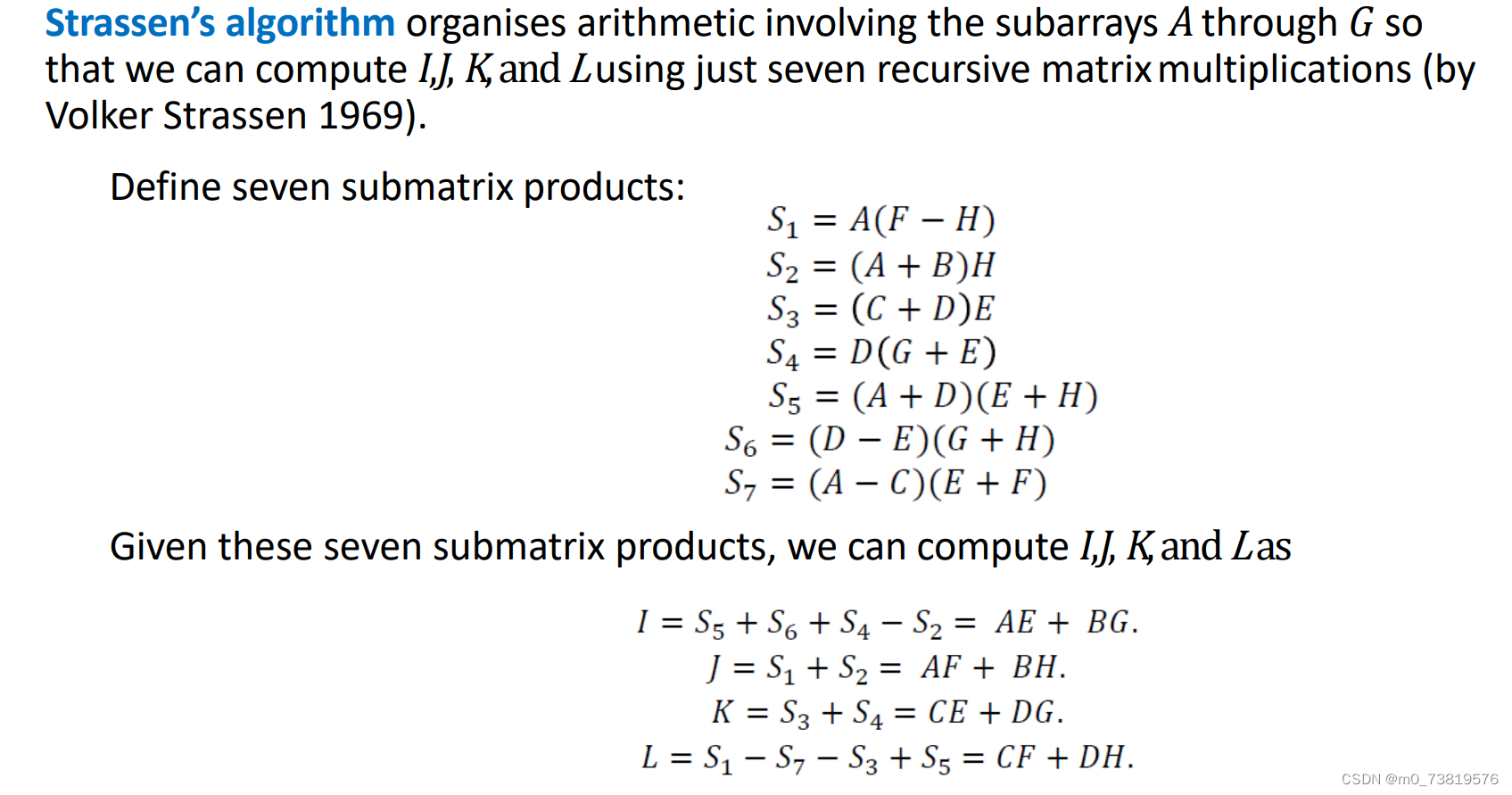

3.3.1 we can compute 𝑍 = X𝑌 using seven recursive multiplications of matrices of size (n/2)×(n/2). Thus，T(n)=7T(n/2)+bn^2(for some constant 𝑏 > 0)

3.3.2 By the master theorem, we can multiply two n x n matrices in 𝑂(𝑛^log7)time using Strassen’s algorithm.

4. Counting inversions

4.1 定义

比较排名，寻找多个排名里与你的排名最相似的数据。 One way is to count the number of inversions.

Suppose that 𝑎1, 𝑎2, 𝑎3, . . . , 𝑎𝑛 denotes a permutation of the integers 1, 2, . . . , n. The pair of integers i , j are said to form an inversion if i < j , but 𝑎𝑖 > 𝑎𝑗. We can count the number of inversions to measure the similarity of someone’s rankings to yours.

eg : 1432里有三对反转，43，32，42

4.2 范围

因为是两两组队,所以反转值范围从0到 $C_{n}^{2}$ = n(n-1)/2

$C_{n}^{m}$ = $A_{n}^{m}$ /m! = n!/(m! (n-m)!)

4.3 时间复杂度

① 挨个查，O(n^2)

② count inversions using a divide-and-conquer algorithm that runs in time O(n log n).

4.4 Divide-and-conquer for counting inversions

① divided the list into A (the first half) and B (the second half) and have counted the inversions in each.这时我们需要计算除了两个子列自己拥有的反转之外的，合并两个子列的额外反转。

② As we merge the lists, every time we take an element from the list B, it forms an inversion with all of the remaining (unused) elements in list A. 额外反转算法

所以不难看出来求额外反转的复杂度是O(n),列被二分logn，所以算法是nlogn

虽然上课应该会讲，但是ppt内容真的好糙...

4.5 In terms of the ranking system describe earlier, the number of inversions for a permutation is a measure of how “out of order” it is as compared to the identity permutation 1 2 3 . . . n and hence could be used to measure the “similarity” to the identity permutation.

Lec6 Complexity of Algorithms Optimization Problems

1.Optimization Problems

1.1定义

Optimization problems can have many possible solutions, and each solution has a value, and we wish to find a solution with the optimal (minimum or maximum) value.

It typically go through a sequence of steps, with a set of choices at each step.

2.Greedy Method

2.1 定义

贪婪算法也是一种优化问题，但是它每一步都是做的局部最优解，不一定能找到全局最优

有贪婪解的问题possess the greedy-choice property

2.2 The Knapsack Problem

2.2.1问题：Let S be a set of n items, where each item i has a positive weight 𝑤𝑖 and a positive benefit 𝑏𝑖 .Find the maximum benefit subset that does not exceed a given total weight (capacity)W.

2.2.2解决：In the solution to an FKP, we use a heap-based priority queue to store items of S, where the key of each item is its value index (vi / wi).所以堆的根处是索引最大值

2.2.3时间复杂度：

①按照贪婪策略，每次尽可能多的拿(vi / wi)最高的物品

②每次贪婪选择（删索引最大）需要O(logn)

③如果最高的拿完了，再去拿下一个，直到W。因此总时间复杂度是O(nlogn)

3.Interval Scheduling

3.1问题：一系列需要时间的任务，你需要最大限度的保证安排任务的数量

3.2解决思路In this case our greedy method would accept a single request, while the optimal solution could accept many. We want to "free up" the machine as soon as possible to start another task.

3.3问题解决：

Order the tasks in terms of their completion times. Then select the task that finishes first, remove all tasks that conflict with this one, and repeat until done.简单来说就是可以按照结束时间对任务进行排序，然后依次选取最早结束的任务，并排除与该任务相交的其他任务。

Furthermore, we can make this algorithm run in time O(nlogn) (the main time will lie in sorting the tasks by their completion times).

3.4Task Scheduling

Now we want to schedule all of the tasks using as few machines as possible (in a non-conflicting way).

首先，我们将任务按照它们的开始时间进行排序，并依次检查每个任务：

如果当前任务可以分配到已有的某台机器上（即不与该机器上的其他任务时间重叠），我们就将该任务安排在这台机器上。
如果当前任务无法分配到任何已有的机器上，那么我们就新分配一台机器，并将任务安排在新的机器上

4.Dynamic Programming

4.1描述

①It is similar to divide-and-conquer. The main difference is in replacing (possibly) repetitive recursive calls by a reference to already computed values stored in a special table.

②It is often applied where a brute force search for optimal value is infeasible.

③dynamic programming is efficient only if the problem has a certain amount of structure that can be exploited.

例子：之前课里学过动态解斐波那契数列，在动态规划中可以通过存储子问题的解来避免重复计算。

4.2Hallmarks:

Optimal substructure: optimal solution to problem consists of optimal solutions to subproblems

Overlapping subproblems: few subproblems in total, many recurring instances of each (a recursive algorithm revisits the same problem repeatedly)还是拿斐波那契举例，避免重复计算

4.3Basic idea and Variations

Idea：Solve bottom-up, building a table of solved subproblems that are used to solve larger ones

“Table” could be 3-dimensional, a tree, etc.Table是指动态规划中用于存储子问题解的数据结构，可以是二维也可以是三维，甚至是树，由问题决定。

5.The {0 – 1} Knapsack Problem

5.1 The {0, 1} Knapsack Problem is the knapsack problem where taking fractions of items is forbidden.

根据公式和已知条件把图列出来找到最优答案

Lec7 Complexity of Algorithms Graphs

1. Graph

1.1 Definition

A graph 𝐺 = 𝑉, 𝐸 consists of a set of vertices V and a set of edges E, where each 𝑒 ∈ 𝐸 is specified by a pair of vertices 𝑢, 𝑣 ∈ 𝑉. (ordered pair ⇒ directed edge of graph ; unordered pair ⇒ undirected)

1.2 Terminology

①End vertices (or endpoints) of an edge ,eg : U and 𝑉 are the endpoints of a

②Edges incident on a vertex , eg : a, d, and b are incident on 𝑉

③Adjacent vertices , eg : U and 𝑉 are adjacent

④Degree of a vertex , eg : 𝑋 has degree 3

⑤Path ：sequence of alternating vertices and edges（Simple path is a path such that all its vertices and edges are distinct）

⑥A spanning subgraph of G is a subgraph of G that contains all the vertices of G.

⑦A graph is connected if, for any two distinct vertices, there is a path between them. If a graph G is not connected, its maximal connected subgraphs are called the connected components of G.

⑧An acyclic graph does not contain any cycles. Trees are connected acyclic graphs； Directed acyclic graphs are called DAGs. it's impossible to come back to the same node by traversing the edges.

2. Pathfinding algorithms

2.1 Breadth First Search

广度搜索从初始点开始，添加当前前沿点的相邻点来扩展前沿

2.2 Depth First Search

从起始顶点开始，沿着一条路径一直走到底，直到无法再继续前进为止，然后回溯到上一个节点，继续搜索其他尚未访问的路径，直到所有的节点都被访问完毕。

2.3 BFS vs DFS

BFS traversal: Finds shortest paths in a graph.

DFS traversal: Produces a spanning tree, such that, all non-tree edges are back edges.所有的非树边都是回边back edges(u, v) such that v is ancestor of node u，可以检测图中的环路

2.4 Cycle Detection

Graph G has a cycle ⇔ DFS has a back edge，简单来说就是最后一个点到初始点的边不在深度搜索形成的树上，该边称为回边，如果存在则说明图是循环的

2.5 Topological Sort

①Order the nodes in a DAG such that there is no path from later nodes to the earlier nodes. eg ：b,f,g,a,c,d,e,h ②Use DFS multiple times, and reverse the popped time of nodes in DFS.简单来说就是利用逆向思维，最先退出DFS的顶点一定是出度为0的顶点，也就是拓扑排序中最后的一个顶点。所以把dfs里的访问结束（也就是pop time）顺序反过来当成我们需要的拓扑顺序，h先结束h是最后

③Proof: If there is a path from a later node to earlier node, there is an edge from a later node to an earlier node. Now, we show no such edge exists. In other words, for any edge (u,v), v finished before u.

拓扑排序的定义要求图中不存在从后面的节点指向前面节点的路径。证明的结论表明在DFS遍历中，任意一条边上前面节点的完成时间早于后面节点的完成时间，这意味着在DFS的过程中，后面的节点会在前面的节点之前完成遍历，从而保证了拓扑排序的性质，也就是不存在从后面的节点指向前面节点的路径。

3. Weighted Graphs

3.1 Definition

A weighted graph is a graph that has a numerical label 𝑤(𝑒) associated with each edge 𝑒, called the weight of 𝑒.

The length (or weigh) of a path 𝑃 is the sum of the weights of the edges 𝑒1, … ,𝑒𝑘 of P.

The distance from a vertex 𝑢 to a vertex 𝑣 in 𝐺, denoted d(u,v) is the value of a minimum length path (also called a shortest path) from 𝑢 to v.

3.2 Single-Source Shortest Paths(SSSP)

For some fixed vertex 𝑣, find the shortest path from 𝑣 to all other vertices 𝑢 ≠ 𝑣 in 𝐺 (viewing weights on edges as distances) which has non-negative weights.

The main idea in applying the greedy method to SSSP is to perform a “weighted” Breadth First Search. One algorithm using this design pattern in known as Dijkstra’s algorithm.

4. Dijkstra’s algorithm

4.1 Time Complexity

O(v) inserts into priority queue

O(v) EXTRACT MIN operations

O(E) DECREASE KEY operation

①Array implementation: O(v) time for extra min

O(1) for decrease key

Total: O(V.V + E.1) = O(V^2 + E) = O(V^2)

②Binary min-heap: O(lg V ) for extract min

O(lg V ) for decrease key

Total: O(V lg V + E lg V )

4.2 Lemma 1:

The relaxation algorithm maintains the invariant that D[u] ≥ d(v, u) for all u ∈ V .

D[u]：表示从源点v到顶点u的最短路径估计值
d(v, u)：表示从源点v到顶点u的实际最短路径长度

Proof: By induction on the number of steps. Consider RELAX(u, z). By induction D[u] ≥ d(v, u). By the triangle inequality, d(v, z) ≤ d(v, u) + d(u, z). This means that d(v, z) ≤ D[u] + w(u, z), since D[u] ≥ d(v, u) and w(u, z) ≥ d(u, z). So setting D[z] = D[u] + w(u, z) is safe.

4.3 Lemma 2：

When u is popped, D[u] ≤ d(v, u) for all u ∈ V . x-y-v-u

Proof : Let’s consider the first u about to be popped（即在Dijkstra算法中作为当前最小距离顶点被处理） that has D[u] > d(v, u). Then, there is a shortest path P can reach u from v that has length d(v,u). In the path, let y being a node that has been popped, and z be a node that has not being popped. y and z exist because v can be y, and u can be z.

Proof continue:(a) D[y] = d(s, y), as y is popped. (b)D[z] ≤ D[y]+w(y, z). As all edges from y has been relaxed. (c) D[u] ≤ D[z], because the pop order (d) d(v, z) = d(v, y) +w(y, z) and d(v, u) = d(v, z) +d(z, u), as P is the shortest path. In all, D[u] ≤ D[z] ≤ D[y] + w(y, z) = d(v, z) ≤ d(v, z) + d(z, u) = d(v, u)

我们认为路径上的每个顶点都会在算法的执行过程中被处理到，而对路径上的顶点进行遍历顺序是无法预知的。因此，假设v可以是y，而u可以是z。再根据pop顺序，得出D[u] ≤ D[z]，再根据定理1的松弛得出D[z] ≤ D[y]+w(y, z) 。（"松弛"操作就是检查是否可以通过（u，v）顶点u缩短v的最短路径估计值D[v]，y出发的边松弛后说明D[z]变小或者不变）

4.4 Shortest paths with negative weights

Re-weighting Add a constant to every edge weight doesn't work.

5. Bellman-Ford algorithm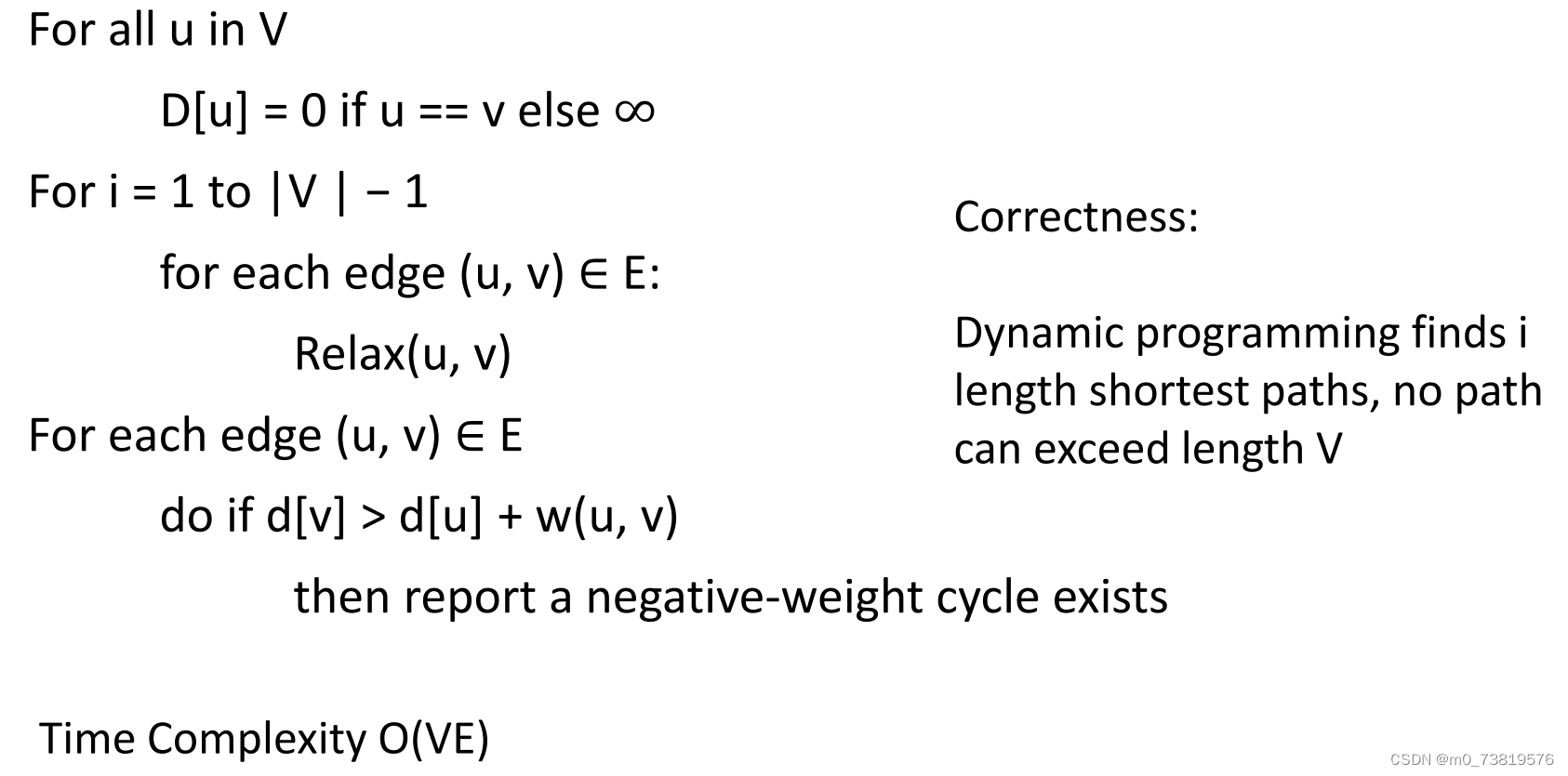

前面和Dijkstra算法一样计算，然后通过检测d[v] > d[u] + w(u, v) 得出是否含有负重的边

6. Minimum Spanning Tree (MST) And Prim’s algorithm

6.1 MST

Let G be an undirected graph. We are also often interested in finding a spanning tree T , i.e. an acyclic spanning subgraph of G, which minimizes the sum of the weights of the edges of T . Such tree is a Minimum Spanning Tree or MST for short.

6.2 Prim’s algorithm

Prim’s algorithm is a greedy type of algorithm designed to find MST

从根顶点开始构建 MST。每一步，我们都会在当前树中没有的顶点上增加一条边，从而 "grow "这棵树，我们会选择一条 "attachment cost "最小的边，同时确保不会与已选的边形成循环。

6.3 Prim’s algorithm pseudocode

U contains the list of vertices that have been visited and V-U the list of vertices that haven't.

T = ∅;
U = { 1 };
while (U ≠ V)
let (u, v) be the lowest cost edge such that u ∈ U and v ∈ V - U;
T = T ∪ {(u, v)};
U = U ∪ {v}

6.4 Prim’s algorithm时间复杂度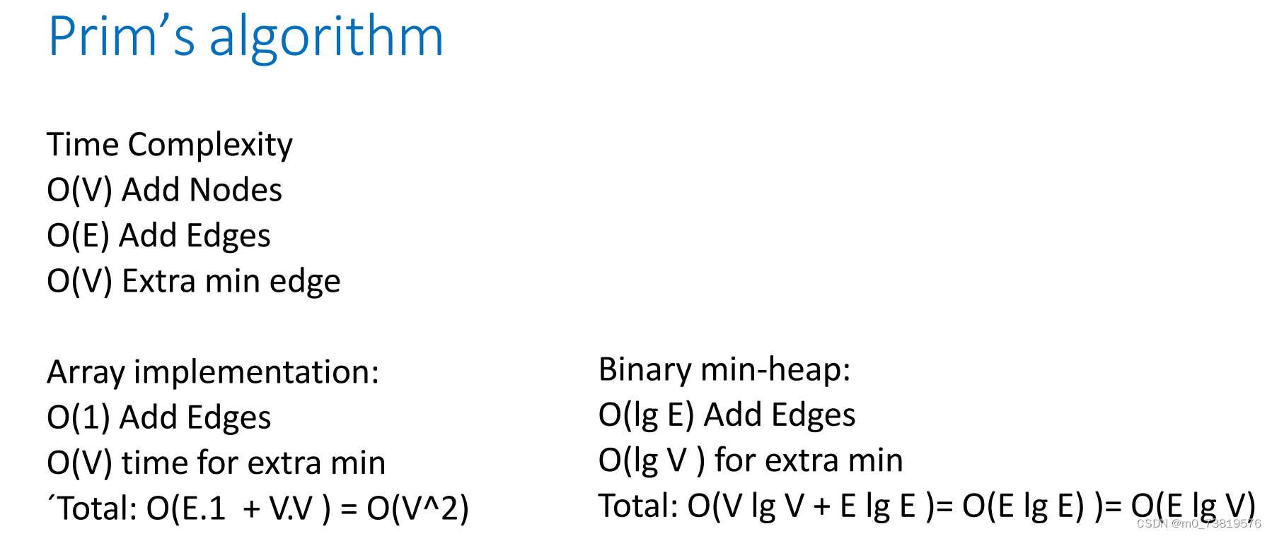

6.5 Kruskal’s Algorithm for MST

Kruskal 算法和 Prim 算法一样，是一种贪婪算法。与 Prim 算法不同的是，Prim 算法是从某个顶点开始 "增长 " ，Kruskal 算法是按从小到大的顺序考虑边，在每一步中，我们都会贪婪地选择最小的边，该边不会与之前选择的边形成循环

Lec11,12 Network Flow and LP Duality

1.Flow Network

1.1 Component

A flow network (or just network) N consists of : ①A weighted digraph G with nonnegative integer edge weights, where the weight of an edge e is called the capacity c(e) ofe. We 0 to c(e) if e is not present.

②Two distinguished vertices, s and t of G, called the source and sink, respectively, such that s has no incoming edges and t has no outgoingedges.

1.2 Definition

A flow f for a network N is is an assignment of an integer value f (e) to each edge e that satisfies the following properties:

① Capacity Rule: For each edge e, 0 ≤ f (e) ≤ c(e)

② Conservation Rule: For each vertex v ≠ s，t, v的出边的流总数 = 入边的流总数

③The value of a flow f, denoted |f|, is the total flow fromthe source,which is the same as the total flow into the sink.

1.3 Maximum Flow

A flow for a network N is said to be maximum if its value is the largest of all flows for N.

The maximum flow problem consists of finding a maximum flow for a given network N

1.4 Cut - Definitions

①A cut of a network N with source s and sink t is a partition X = (S, T) of the vertices of N such that s ∈S and t ∈ T ：

Forward edge of cut X: origin in S and destination in T

Backward edge of cut X : origin in T and destination in S

②Flow f (X) across a cut X: total flow of forward edges minus total flow of backwardedges

③Capacity c(X) of a cut X: total capacity of forward edges

eg：两个直观的例子

1.5 Flow and Cut

① Lemma 1: Let N be a flow network, and let f be a flow for N. For any cut X of N, the value of f is equal to the flow across cut X , that is, |f| = f(X).

Proof: Induction on cuts. The base case is the cut ({s},X-{s}). Any other cuts can be obtained by moving node from S to T one by one.

②Lemma 2: Let N be a flow network, and let X be a cut of N. Given any flow f for N, the flow across cut does not exceed the capacity of X, that is, f (X) ≤ c(X).

③Theorem 1: The value of any flow is less than or equal to the capacity of any cut, i.e., for any flow f and any cut χ,we have |f | ≤ c(χ).

⇒ The value of a maximum flow is no more than the capacity of a minimumcut.

1.6 Augmenting Path and Residual Network

降低流的值来改变流

增广路径，就是找到一条流量不满，未达到容量上限的一条路径

Residual capacity ：∀ u, v ∈ E ，cf (u, v ) = c (u, v) – f (u, v), cf (v, u) = f (u, v) 简单来说每条弧的残留容量表示该弧上可以增加的流量，每条弧 <u,v> 上还有一个反方向的残留容量 cf (v,u) = - f(u,v)，路径的残留容量是路径上某边的最小残留容量

2.The Ford-Fulkerson Algorithm

2.1 算法

Initially, f(e) = 0 for each edge e

Repeatedly until no augmenting path ▷ Search for an augmenting path p ▷ Compute bottleneck capacity cf(p) ▷ Increase flow along the edges of p by bottleneck capacity cf (p) 找出一条从 s 到 r 的不定向路径，使得可以增加前向边缘的流量（非满); 能减少后向边缘的流量（非空）。直到从 s 到 r 的所有路径都被 "满前向边 "或 "空后向边 "阻断。

从源点S到汇点T的一条路径中，如果边(u,v)与该路径的方向一致就称为正向边，否则就记为逆向边，如果在这条路径上的所有边满足：正向边f(u,v)<c(u,v)；逆向边f(u,v)>0，则该路径是增广路径

2.2 Flow Integrality

Theorem: If the flow network has integer capacities, the maximum flow will be integer-valued and Ford-Fulkerson terminate

Proof:每一步FF都会找残留容量为整数的增强路径，因此边的流量值始终为整数。每次更新都会让流量值增加至少一，而且流量值有上限，所以FF最终停止

3. Max-flow, min-cut theorem

3.1 Definition

The following are equivalent: ①. |f| = c( S, T) for some cut ( S, T). ②. f is a maximum flow. ③. f admits no augmenting paths.

Proof ①⇒ ②: Since | f | ≤ c ( S, T) for any cut ( S, T), the assumption that | f | = c ( S, T) implies that f is a maximum flow.

②⇒③: If there were an augmenting path, the flow value could be increased, contradicting the maximality of f

③⇒ ①: We need to construct a cut such that |f| = c( S, T) . Let S = {s} ∪{v ∈ V : there exists a path in 𝐺𝑓 from s to v }, and T=V-S. As no augmenting path from s to t exists, t does not belong to S. So, (S,T) is a cut. ∀u ∈ S and v ∈ T, we must have cf(u, v) = 0, since if cf ( u, v) > 0, then an augmenting path from s to v exists. Note that cf (u, v) = c ( u, v) – f ( u, v )=0. So, f ( u, v) = c ( u, v ).Furthermore, if there is backward edge flow from T to S, there will be another augmenting path and at least one node in T should be in S. So, ∑𝑢∈𝑆,𝑣∈𝑇 𝑓(𝑣, 𝑢) = 0

4. Bipartite Matching

4.1 Definitions

①A graph G = (V,E) is called bipartite if and only if the set V can be partitioned into two sets（X and Y） or Every edge of G has an endpoint in X and the other endpoint in Y.

②A matching M ⊆ E is a set of edges that have no endpoints in common. Each vertex from one set has at most one "partner" in the other set.

③If a vertex v has no edge of M incident to it then v is said to be exposed (or unmatched)). ④A matching is perfect if no vertex is exposed.

4.2 Maximum Bipartite Matching

The maximum bipartite matching problem is to find a matching M with the greatest number of edges (over allmatchings).

Given a bipartite graph G = (A ∪B ,E ), find an S ⊆ A × B that is a matching and is as largeaspossible. A maximal bipartite matching is the largest subset of edgesin a bipartite graph such that no two selected edges share a common vertex.不保证唯一性

4.3 Reduce

We can solve the maximum bipartite matching problemusing a network flow approach.保证边是有向边，加一个源点和汇点，得到一个无权有向图

Solving maximal flow for an unweighted directed graph:

① Construct the directed graph with a source and sink node.

② Using a search method to find a path from the source to the sink.

③ Once a path is found, reverse each edge on this path.

④ Repeatstep2 and 3 until no morepaths from the sourceto sinkexist.

⑤ The final matching solution is then the set of edges between U and V that arereversed(i.e. run from V to U).

Lec13 Number Theory and Cryptography

1. Security of Communications

1.1 Cryptography

Encryption needs to be injective so that decryption is possible

Encryption take parameters (keys) so that it is not always the same

Decryption take parameters (keys) so that it matches the varying encryption

1.2 Symmetric encryption schemes and secret keys

Caesar cipher: each character x is replaced by the character y = (x + k ) mod n, where n is the size of the alphabet andthe integer k , 1 ≤ k < n, is the secret key

举例：Alice把密钥k=3发给Bob，Bob把消息“Hello World”加密为“Khoor Zruog”发给Alice，Alice便可以解密Khoor Zruog得到Hello World。

1.3 The One-time pad

The most secure cipher known is the symmetric cipher that’s referred to as the one-time pad.这种加密方式双方共享一个随机比特串K，K与双方要发送的任何消息一样长。K就是加密解密的对称密钥，并且K要大于等于信息密钥。密钥必须是一次性的，每次随机生成。

①encryption：To encrypt M，C = M ⊕ K, where the ⊕ symbol denotes the bitwise “exclusive-or” （不同为一）operation.因此C也变成了一种随机比特串，ci = (mi+ki) mod 2

②decryption：C ⊕ K = (M ⊕ K) ⊕K = M ⊕(K ⊕ K) = M ⊕ 0 = M，where 0 represents the all-zero string with the same length as M.

③优劣：优势是Computationally efficient ，Very secure

劣势是must share a very long keyK，Security depends on the fact that the key is used only once

2. Public-key cryptography

2.1 起源

因为对称加密的问题是如何安全的分配密钥，于是出现了公共密钥加密系统

2.2 Public-key cryptography system

A public-key cryptosystem consists of an encryption function E and a decryption function D. For any message M, the following properties musthold:

①D(E(M)) = M. ②Both E and D are easy to compute. ③It is computationally infeasible to derive D from E.

因此除了解密D的持有者，任何人有E但都不知道D，所以任何人都能用E给持有者发信息。For this reason E is referred to as a one-way function.

3. INTEGER ARITHMETIC

3.1 整数集，除

Z={... -2,-1,0,1,2,...}

除法视为a = q × n + r ,0 ≤ 𝑟< |𝑛|。a为正数，r非负；a为负数，q和r都为负数

If the remainder is zero, 𝒏| a

If the remainder is not zero, 𝒏∤ a

3.2 Property

① if a|1, then a = ±1.

② if b|a and a|b, then a = ±b.

③ if b|a and c|b, then c|a.

④ if a|b and a|c, then a| (m × b + n × c), where m and n are arbitraryintegers

举例：3|15，15|45，所以3|45；3|9，3|15 所以 3|（9*2+15*2）=3|48

3.3 Greatest Common Divisor

The greatest common divisor of two positive integers is the largest integer that can divide both integers

3.4 EuclideanAlgorithm

①Lemma: Let a, b, q, and r be integer such that a = bq + r and 𝒃 ≠ 𝟎. Then gcd(a, b) = gcd(b, r) = gcd(b, a % b). 这里gcd（a，b）就是指最大公约数，特殊gcd (a, 0) = a

②Proof. Let d = gcd(a, b) and e = gcd(b, r). We need to show that d = e. Since d|a and d|b, 所以d也能够整除它们的线性组合，即d divides a − bq = r. So d is a common divisor of b and r. Hence d ≤ e. Similarly, as e|b and e|r, e divides bq + r =a. Thus, e is a common divisor of both a and b, so e ≤ d. This proves that d = e.

When gcd (a, b) = 1, we say that a and b are relatively prime.

举例：Given 26 = 6 × 4 + 2 ,find the gcd (26,6) and gcd(6,2).

Solution a=26 , b=6, r=2 ，common divisors of 26 and 6: (1,2) ，common divisors of 6 and 2: (1,2) ，gcd(a,b)=2, gcd(b,r)=2

③代码：

def gcd(a,b) 
    assert a>=b and b>=0 and a+b>0 
    return gcd(b, a%b) if b>0 else a

3.5 Extended Euclidean Algorithm

Given two integers a and b, we often need to find other two integers, s and t, such that

s * a+ t * b = gcd(a,b), 在计算gcd的同时能得出s和t。

举例：从下往上推导就行

4. MODULAR ARITHMETIC

4.1 Modulo Operator

The modulo operator is shown as mod (or % in some languages). The second input (n) is called the modulus. The output r is called the residue.

4.2 Set of Residues

The modulo operation creates a set, which in modular arithmetic is referred to as the set of least residues modulo n, or Zn. Zn = {0,1,2,...,n-1}

4.3 Congruence

To show that two integers are congruent, we use the congruence operator ( ≡ ): a≡b(mod m) a is congruent to b modulo m.

A residue class [a] or [a]n is the set of integers congruent modulo n: {… , a − 3n, a − 2n, a − n, a, a + n, a + 2n, a + 3n, …}.

举例：2≡12(mod 10) ；-8≡2≡12≡22(mod 10)

4.4 Operation in Zn

The three binary operations that we discussed for the set Z can also be defined for the set Zn. The result may need to be mapped to Zn using the mod operator.

Properties of mod operator：

①First Property: (a + b) mod n = [(a mod n) + (b mod n)] mod n
②Second Property: (a-b) mod n = [(a mod n) - (b mod n)] mod n

③Third Property: (a x b) mod n = [(a mod n) x (b mod n)] mod n
④Fourth Property: a^n mod b = (a mod b)^n mod b 其实是直接来源于③

举例：10^n mod 3 = (10 mod 3) ^n mod 3 = 1^n mod 3=1

4.5 Inverse

①Additive Inverse：In Zn, two numbers a and b are additive inverses of each other if a+b ≡ 0 (mod n). 注意对于任意整数a，都存在一个加法逆元（-a），也可能有多个

②Multiplicative Inverse：In Zn, two numbers a and b are the multiplicative inverse of each other if a x b ≡ 1 (mod n). 但是对于任意正数，是可能有一个乘法逆元

ab=1+nq，ab-qn=1=gcd(b,n) , so we can use the extended Euclidean algorithm to find a. The multiplicative inverse of b is the value of t after being mapped to Zn. b的乘法逆元表示为 $b^{-1}$ (mod n)

举例：Find the multiplicative inverse of 11 in Z26. 𝑠 × 𝑛 + 𝑡 × 𝑏 = gcd 𝑛, 𝑏 = 1

The multiplicative inverse of 11 modulo 26 is 26-7=19.

4.6 Different Sets

We need to use Zn when additive inverses are needed; we need to use Zn* when multiplicative inverses are needed.简单来说就是Zn*由Zn里能gcd(a,n)=1的元素组成，例如Z10* = {1,3,7,9}

Cryptography often uses two more sets: Zp and Zp*. The modulus p in these two sets is a prime number.

4.7 Fast Modular Exponentiation：

3^94(mod 17) ,94=64+16+8+4+2=1011110 = 101111*2+1

n = 2* d + r (r = 0 or 1) 所以我们可以得出a^n (mod b) = (a^r mod b) * (a^d mod b)^2 (mod b)

此时3^94（mod 17） =

If a is an integer, p is a prime number and a is not divisible by p, then a^(p-1) ≡ 1 (mod p) or equivalently a^p ≡ a (mod p)

4.8 Euler’s Theorem

Lec14 Number Theory and Cryptography

1. Public-key cryptosystems

1.1 Turing’s Code

使用公开密钥e,n对明文M进行加密：C ← M*e mod n.

解密也是 by modular multiplication: M ← C*d mod n. If d ≡ e^-1 mod n, the scheme can transmit messages.但是也太容易被计算出乘法逆，所以不安全。

1.2 Desiderata of RSA

使用公开密钥e,n对明文M进行加密：C ← M^e mod n.

解密也是 by modular multiplication: M ← C^d mod n. Can we choose e, n, and d, such that for every integer 0 ≤ 𝑥 < 𝑛 we have x^(ed) ≡ x mod n.

1.3 Euler’s Theorem

Let 𝑛 be a positive integer. If 𝑎 is an integer such that gcd 𝑎, 𝑛 = 1, then a ^ ϕ(n) ≡ 1 mod n

Corollary: Let 𝑛, 𝑘 be a positive integers. If a is an integer such that gcd (a, n)= 1, then a^(kϕ(n) +1) ≡ a mod n. So de = kϕ (𝑛) + 1.If we further assume gcd( 𝑒,𝜙(𝑛)) = 1, finding d becomes finding multiplicative inverse of 𝑒 mod 𝜙(𝑛) . So, we have found a commutative encoding and decoding method.

We know that given ϕ (𝑛) , the solution can be found by the extended Euclidean algorithm. So, we must choose n such that ϕ (𝑛) is hard to compute. Recall that ϕ (𝑛) can be computed by factorizing n. Therefore, we must choose n that is hard to factorize.

The first step is to select two large prime numbers p and q. Let n = p·q and define ϕ(n) = (p − 1)(q − 1). We then choose two numbers e and d such that ① e and ϕ(n) are relatively prime, so that e has a multiplicative inverse modular ϕ(n) i.e., de = kϕ (𝑛) + 1 has solution ② de ≡ 1 (mod ϕ(n)) (by Extended Euclidean algorithm)

1.4 Digital signatures

RSA 密码系统支持数字签名。假设 Bob 向 Alice 发送了一条信息 M，而 Alice 想要确认
是 Bob 发送的。鲍勃可以 M= I’m Bob : S ← M^d mod n.

同样的Alice可以用加密函数验证签名：M ≡ S^e (mod n).

1.5 Breaking RSA

对n因式分解可以得到ϕ(n),但是太难了

Theorem: Let n = pq be an RSA modulus with |p − q| < c × 𝑛^1/4 where c is a positive constant. Then one can factor N in time polynomial in c.

即使是大n，Shor’s Factoring Algorithm solves the factoring problem with bounded error probability in polynomial time.

Lecture15 NP-Hardness and Language

1. Decision/Optimization problems

1.1 The {0, 1} Knapsack problem

The dynamic programming algorithm for the { 0,1} Knapsack problem runs in time θ(nW), which is not polynomial in the size of the problem.

1.2 Decision/Optimization problems Definition

A decision problem is a computational problem for which the output is either yes orno. In an optimization problem we try to maximize or minimize some value. An optimization problem can often be turned into a decision problem by adding a parameter k, and then asking whether the value of the function (from the optimization problem) is at most or at least k.

If a decision problem is hard, then its related optimization version must also be hard.

例子：Is there a subset of the items whose total weight does not exceed W, and whose total benefit is at least k?如果能高效的解决决策问题，则可以高效的解决优化问题

1.3 Problems and Language

The input to a computational problem will beencoded as a finite binary string s. The length of the string is denoted as |s|.

We identify a decision problem with a set of strings for which the answer is “yes”. We say that the algorithm A for the decision problem accepts an input string s if A outputs “yes” on input s.

For some decision problem X , let L(X) denote the set of (binary) strings that should be accepted by an algorithm for that problem. We often refer to L(X) as a language. • We say that an algorithm A accepts a language L(X) if A outputs “yes” for each s ∈ L(X) and outputs “no” otherwise.

1.4 Language Examples

Now consider the {0,1} Knapsack Problem (the decision version). The encoding of the problem will be the binary representations of the integer weights { wi }, benefits {bi}, the maximum weight W , and the parameter k. (It takes log2 k bits to represent an integer k.)

1.5 Complexity Class P

The complexity class P is the set of all decision problems X that can be solved in worst-case polynomial time. (Equivalently, P consists of all languages L(X) that can be accepted in polynomial time.)也就是可以在O(p(n))内被解决 , p(n)是n的多项式；确定算法本质上是总能计算出正确答案的算法

P类中包括fractional knapsack, shortest paths in graphs with non-negative edgeweights, task scheduling.

1.6 Efficient certification

The Sudoku decision problem is whether a given Sudoku problem has a solution. Finding the solution might be difficult, but verifying the solution is easy.简单来说就是你给问题一个项目子集，它可以很轻松的验证项目子集是不是问题的解

the subset of items is a certificate for the decision problem, i.e. it verifies that the answer to the { 0,1} Knapsack decision problem is “yes.” The idea of efficient certification is what is used to define the class of problems called N P.

1.7 Complexity class NP (non-deterministic polynomial time)

The class N P consists of all decision problems forwhich there exists an efficient certifier.

An efficient certifier for a decision problem X is an algorithm B that takes two input strings s and t . The string s is the input to the decision problem. “efficient”意味着B是一个多项式时间算法，也就是说存在一个多项式函数q(·)，对于每个字符串s，如果存在一个字符串t使得|t| ≤ q(|s|)并且B(s,t) = “yes”，那么s ∈ L(X)，即在决策问题X中返回“yes”，t是一种证明（|t| ≤ q(|s|) 限制证明字符串t的长度，使其不会太长。这样的限制是为了确保有效验证器B的运行时间在多项式级别）

A non-deterministic Oracle that make multiple certificates, and let the algorithm ends once one certificate got certified.

An algorithm that executes some number of non-deterministic branches during its execution is calleda non-deterministic algorithm. It ends when one of the branch ends.

类 N P 是决策问题 X（或语言 L(X)）的集合，这些问题可以在多项式时间内被非确定地接受。因此，NP 也可以看作是一类其解决方案可以在多项式时间内得到验证的问题。

举个例子：

1.8 P and N P

P ⊆ N P . Basically, if there is a polynomial-time algorithm A to solve a problem, then we can “ignore” any proposed solution t.

1.9 Polynomial-time reducibility

称一个语言L（定义了某个决策问题）可以在多项式时间内归约到另一个语言M，如果满足以下条件：存在一个可以在多项式时间内计算的函数f，它接受输入s ∈ L，并将其转换为输入f(s) ∈ M，使得s ∈ L当且仅当f(s) ∈ M。换句话说，我们可以将一个决策问题的输入转换为另一个决策问题的适当输入。当第二个问题有答案了，第一个问题也有了。

这意味着我们可以利用一个问题的解来解决另一个问题。如果我们能在多项式时间内将问题L的实例转换为问题M的实例，并且保持解的性质，那么问题L可以在多项式时间内归约到问题M。

L → （poly）M

1.10 N P-hardness

一个语言M（定义了某个决策问题）是NP-难度（NP-hard），如果每个属于NP的其他语言L都可以在多项式时间内归约到M。也就是说，对于语言M来说，多项式时间内可以将NP中的任何语言L归约到M。

1.11 N P-complete

如果一个语言M是NP-hardness并且它本身属于NP，那么M就是NP-完全（NP-complete）

If an NP-complete problem can be solved in polynomial time, then all problems in NP can be solved in polynomial time, and thus P = NP

证明X是NP-complete ：►First, show that X ∈ NP, i.e. show that X has a polynomial-time nondeterministic algorithm, or equivalently, show that X has an efficientcertifier.

►Secondly, take a known NP-hard problem Y , and demonstrate a polynomial time reduction from Y to X , i.e. show that Y → X.

Lec16 NP-Completeness and the Cook–Levin Theorem

1. SAT

1.1 Definition

SAT: A Boolean formula φ is satisfiable if you can assign truth values to 𝑥1, … , 𝑥𝑛 so that φ(𝑥1, … , 𝑥𝑛) is true. E.g, (𝑥1 ⋁𝑥2 ) ∧ (𝑥3 ⋁𝑥2).这里的x都是布尔值，or和and是|与&

1.2 Vertex Cover (VC)

Given a graph G = (V,E). A vertex cover is a subset C ⊆ V such that for every edge (v,w) in E, v ∈ C or w ∈ C

Vertex Cover is the decision problem that takes a graph G andan integer k and asks whether there is a vertex cover for G containing at most k vertices

①Lemma: VC is in NP

Proof：Verifying a subset selection of size k (as certificate) that is a valid cover only requires enumerating over all edges and check whether one of its’ end point is in the cover. Clearly, this takes O(V+E) time.

②Theorem: VC → （poly）SAT

2. Turing Machine

2.1 Definition

On input 𝑤𝑤 a TM 𝑀 may halt (enter 𝑞acc or 𝑞rej) or 𝑀𝑀 may run forever (“loop”).TM在循环和读取到qrej的结果都是Reject，只有读qacc才是Accept.

2.1 Simulate Turing Machine

Theorem: All problems in P can be reduced to SAT

As problems are in P, let n be the length of input. TM finish in polynomial steps O(n^k), this also implies the tape won’t exceed O(n^k) , and the |Q ∪ Γ| is constant. We have polynomial many Xt,i,s .然后构造出Xt,i,s的表达式，因为Xt,i,s只有一个值，于是可以构造出一个表 In each time step, we keep track of position of the head and update information only row by row. So, the completion of the table takes at most polynomial time. Finally, we accept if and only if the last row has one 𝑞accept. This can be done by checking ⋁𝒕,𝒊 (X𝑡,i,𝑞accept).

2.3 𝜙all

2.4 𝜙init

2.5 𝜙move

3. Nondeterministic Turing Machine

3.1 Definition

4. Cook-Levin Theorem

4.1 Theorem

𝑆𝐴𝑇 is NP-complete

Proof: 1) 𝑆𝐴𝑇∈NP：NTM record all seen variables in a simulated working tape and non-deterministically generates all assignments, then verify them. Alternatively, certifying a solution is equivalent to evaluation, which can be done in linear time to the formula size.

Proof: 2) Show NP problems can be polynomial time reduced to SAT

4.2 CNF-SAT and 3-SAT

合取范式（ conjunctive normal form (CNF)）任何命题公式，最终都能够化成(A1∨A2)∧(A3∨A4)的形式，这种先 ∨ 析取再 ∧ 合取的范式，被称为 “ 合取范式”。3合取范式”就是每个子句恰好由3个变量A(eg：b!)所组成的合取范式。每个子句的三个变量至少满足一个

4.3 Vertex Cover (VC) and Hamiltonian Cycle

Lec17 Reduction and Approximation

1. Vertex Cover is NP-Hard

1.1 Definition

Defn: Given an undirected graph G, is there a set C of (at most) k vertices such that every edge of G is incident to at least one node of C ?

1.2 Reduction Goal

In polynomial time, construct a graph and choose k such that a k-vertex cover exists if and only if 3SAT can be satisfied. Idea: 𝜙 = (𝑥1 ⋁𝑥1 ⋁𝑥2) ∧ (!𝑥1 ⋁!𝑥2 ⋁!𝑥2) ∧ (𝑥1 ⋁𝑥2 ⋁𝑥2)

use node selection to represent truth assignment of variable

①Step1 : One node per literal (𝑥𝑖 and !𝑥𝑖 ) and connect them. To cover the edge one of them has to be selected.

②Step 2: For each clause, connect those literals. We need to take at least 2 nodes to cover edges.

③Step 3: Connect the same nodes between variables and clauses.

每个子句需要选择两个节点才能覆盖所有边；每个变量对中需要选择一个节点来覆盖它们之间的边。 Interpreting un-selection in clauses as truth assignment and selection in variables as truth assignment