INT202 算法复杂度 笔记

week01

伪代码，时间复杂度，空间复杂度，平均复杂度与最差复杂度

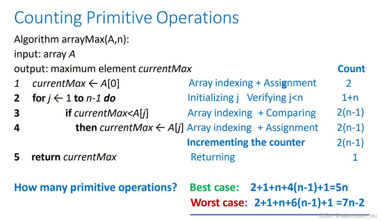
Counting Primitive Operations：数伪代码中的原子操作（每行代码执行多少次）

Recursive Algorithms：递归算法（我调用我自己

1. Asymptotic notation渐进表示（时间复杂度

Used in a simplified analysis that estimates the number of primitive operations executed up to a constant factor

1.1. Asymptotic Algorithm Analysis:渐近算法分析

use the worst-case number of primitive operations executed as a function of the input size

Example:
• We determine that the algorithm “Maximum-Element(A) ” executes at most 7n - 2 primitive operations
• We say that algorithm “runs in O(n) time”

Since constant factors and lower-order terms are eventually dropped anyhow, we can disregard them when counting primitive operations

• Growth rate： Linear ≈n , Quadratic ≈ n²,Cubic ≈ n³,只被最高项所影响: 10²𝑛+10⁵ is a linear function, 10⁵𝑛²+10⁸𝑛 is aquadratic function

1.2. Big-Oh渐进上界:

we say f (n) is O(g(n)), written f (n) ∈O(g(n)), if there are constants c and n₀ such that:
f (n) ≤ c ·g(n) for all n ≥ n₀
存在某一定值c，使得输入参数n大于某一个定值n₀后，fn小于c倍的g(n)我们就说fn∈O(g(n))，算法最坏不超过c·g(n)

结合growth rate来看，还需符合the growth rate of f(n) is no more than the growth rate of g(n).

简单来说，对于多项式f(n)，其大O为f(n)中的最高项（不含系数
13𝑛³+ 7n log n + 3 is O(_ 𝑛3_).Proof: 13 𝑛³+ 7n log n + 3 ≤ 16 𝑛³, for n ≥1

1.3. big-Omega渐进下界:

We say that f (n) is Ω(g(n)) (big-Omega) if there are real constants c and n₀ such that:
f (n) ≥ cg(n) for all n ≥ n₀
存在某一定值c，使得输入参数n大于某一个定值n₀后，fn大于c倍的g(n)我们就说fn∈Ω(g(n)), 算法最优不少于c·g(n)

1.4. Θ(g(n))：

g(n)既是渐进上界也是渐进下界

ref：论文中的一些符号
ref：时间复杂度

2. Space Complexity

That means how much memory, in the worst case, is needed at any point in the algorithm. we‘re mostly concerned with how the space needs grow, in big-Oh terms, as the size N of the input problem grows.

int sum(int a[], int n) {
int r = 0;
for (int i = 0; i < n; ++i) {
r += a[i];
}
return r;
}

Requires N units for a, plus space for n, r and i, so it’s O(N).

Week02

栈stack，
队列queue，
循环队列circlular queue，
列表list，
链表link list，
双向链表double link list

以前数据结构的笔记

Week03

1. 树形结构

同一父节点的子节点之间被称为siblings

1.1. 二叉树Binary tree

A binary tree is a rooted ordered tree in which every node has at most two children. Each child in a binary tree is labeled as either a left child or a right child.

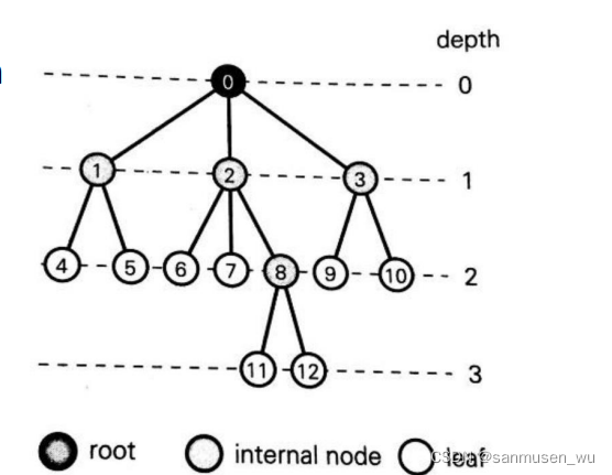
1.2. 获取树某一节点的深度

采用递归的方法
The depth of a node, v, is number of ancestors of v, excluding v itself. This is easily computed by a recursive function.

depth(T,v):
  if T.isRoot(v):
    return 0
  else return 1+depth(T,T.parent(v))

1.3. 获取树的高度

也就是所有叶子节点的最大深度
The height of a tree is equal to the maximum depth of an external node in it.

height(T,v):
  if isEXTERNAL(v)
    then return 0
    else 
      h=0
      for each∈T>CHILDREN(v)
        do
          h=MAX(h,HEIGHT(T,w))
      return 1+h

1.4. 树的遍历Tree Traversal

1. Preorder前序：按照 当前节点-左子树-右子树

preOrder(v):
  visit(v)  //当前节点
  for each child w of v: //左子树-右子树
    preOrder(w)

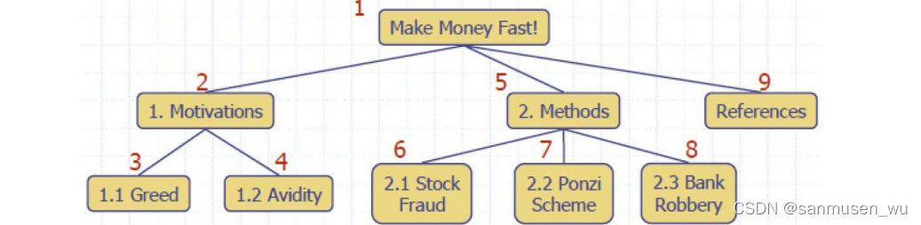
2. Postorder后序：按照 左子树-右子树-当前节点
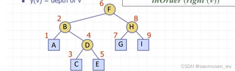
3. Inorder中序：按照 左子树-当前节点-右子树

inOrder(v):
  if hasLeft(v)  //左子树
    inOrder(left(v))
  visit(v)  //当前节点
  if hasRight(v)  //右子树
    inOrder(right(v))

1.5. Parsing arithmetic expressions

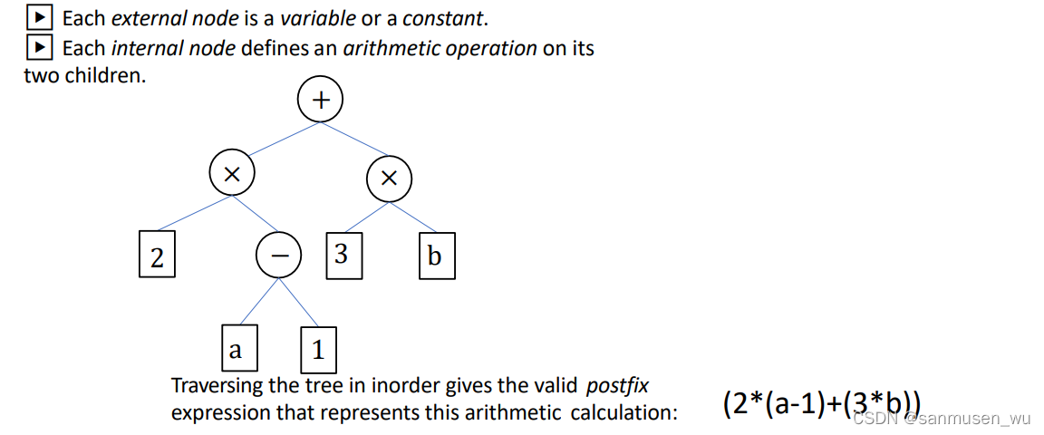
PPT里有误，应该是中序得中缀

1.6. 树的数据结构

Link structure：each node v of T is represented by an object with references to the element stored at v and positions of its parents and children
链表结构，既节点直接互相保存对方的reference，达到关联的效果。

Array structure: For rooted trees where each node has at most t children, and is of bounded depth, you can store the tree in an array A
数组结构举例，对于二叉树，根节点为list[0],左节点list[1],右节点list[2],每一个节点都按照层序的顺序一层一层摆在数组里面

1. In general, the two children of node A[i] are in A[2 ∗ i + 1] and A[2 ∗ i + 2].
2. The parent of node A[i] (except the root) is the node in position
   A[⌊(i − 1)/2⌋].

2. Ordered Data

本节讨论在存储时存储顺序

2.1. Ordered Dictionary

有序字典的键值对按照键的值进行排序，直接把键放在vector里面比放在链表里后续访问会快（vector可以直接根据地址访问元素）
A lookup table is a dictionary implemented by means of a sorted sequence
We store the items of the dictionary in an array-based sequence, sorted by key

2.2. Binary Search

二分搜索
根据区间S，S左边界low，右边界high，
假设一个item对应的key位于i，则i-1以下的key都不大于该key，i+1以上的key都不小于该key

BINARYSEARCH(S, k,low,high)
//Input is an ordered array of elements.
//Output: Element with key k if it exists, otherwise an error.
1 if low > high
2     then return NO_SUCH_KEY // Not present
3 else
4     mid ←mid = ⌊(low + high)/2⌋
5     if k = key(mid)
6         then return elem(mid) //Found it
7     elseif k < key(mid)
8         then return BINARYSEARCH(S, k,low,mid-1) // try bottom ‘half’
9     else return BINARYSEARCH(S,k,mid + 1,high) //try top ‘half’

学校给的是双闭区间，此外还有半开和双开区间的写法

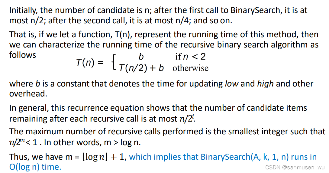
2.3. Complexity of Binary Search

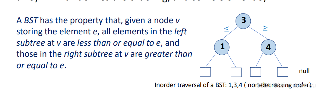
Binary Search Tree

二叉搜索树
假设一个节点值为v，则其左子树的节点的值都不大于v，其右子树的节点的值都不小于v

查找：

findElement(k,v):
  if T.isExternal(v)
    return no such key
  if k<key(v)
    return findElement(k,T.leftChild(v))
  else if k=key(v)
    return element(v)
  else if k>key(v)
    return findElement(k,T.rightChild(v))

其查找的时间复杂度取决于所查找元素的深度，平均O(logn)，最坏O(n)，最差情况BST会退化（ degenerate tree）成单侧树也就是链表

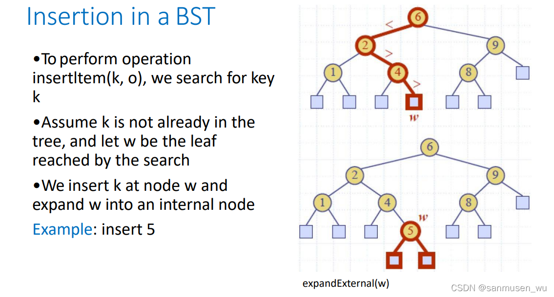
插入：

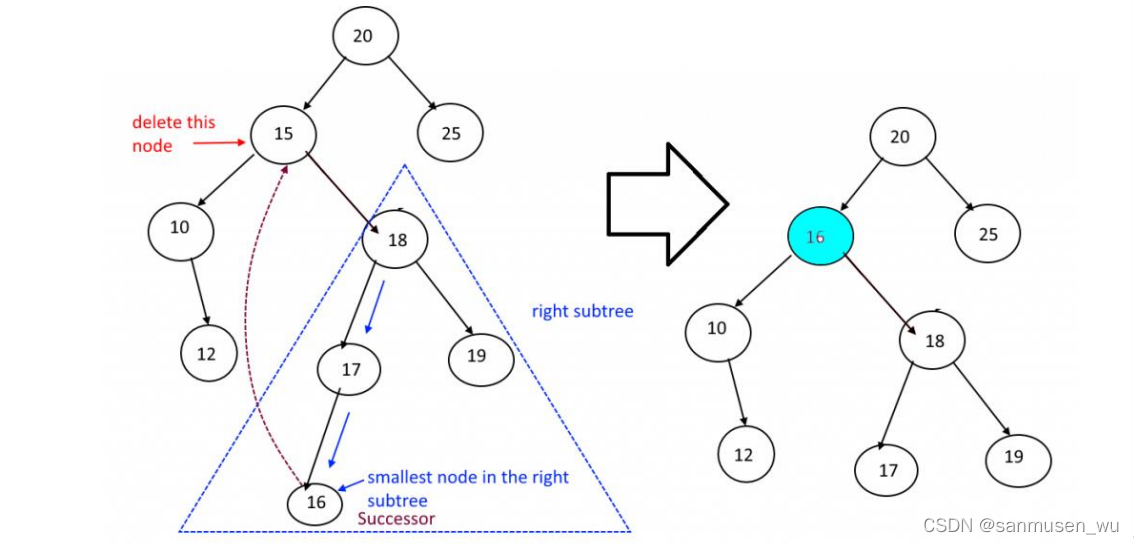
删除：

1. Find the node to be removed. We’ll call it remNode.
2. If it’s a leaf, remove it immediately by returning null.
3. If it has only one child, remove it by returning the other child node.
4. Otherwise, remove the inorder successor of remNode, copy its key into remNode, and return remNode. (inorder successor: the node that would appear after the remNode if you were to do an inorder traversal of the tree)

先找到预删除节点remNode，然后分类讨论
如果是叶子节点，直接删除
如果只有一个子节点，把子节点移动到remNode所在位置
如果有两个子节点，找到其最大继承人/右子树中最小的节点（对整棵树做中序遍历，出现在remNode后面的那个节点，或对remNode的右子树做中序遍历最先遍历到的那个节点）

AVL tree 平衡二叉树

为了解决上述问题，对二叉树形状进行高度平衡约束(height-balance)，以保证查找稳定在O(logn)，而相对应的存删操作变复杂了。

对于任意节点n，其左子树的高度与右子树的高度相差最大为1

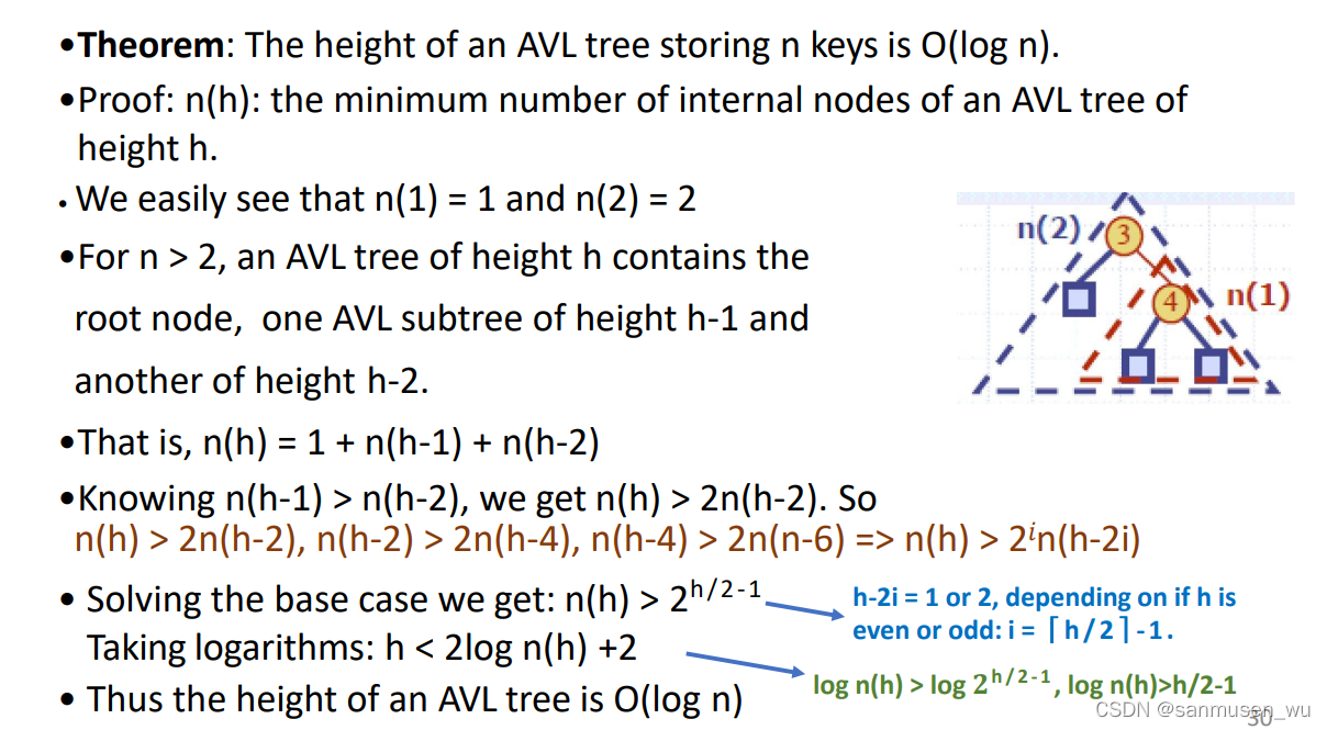
Theorem：存储了n个节点的AVL的高度为O(log n)
n(h): the minimum number of internal nodes of an AVL tree of height h.
Proof：n=1高度1，n=2高度2，设任意n>2的AVL的高度为h，根节点的左子树高度为h-1，右子树高度为h-2。
则高度为h时的最少节点数量n(h)=1+n(h-1)+n(h-2)
易知 n(h-1)>n(h-2), 那么上式 n(h)>n(h-1)+n(h-2)>2n(h-2), 根据递推式进一步推算:
n(h-2)>2n(h-4),n(h-4)>2n(n-6) ==> n(h)>2ⁱn(h-2i)
当h-2i为1或2时得到base case，此时: i = ⌈ h / 2 ⌉-1, 可进一步得到 n(h)>2^h/2-1
取log，得log(n(h))>h/2-1, h<2log(n)+2，证得h < clogn for any n>2,c=2，既O(logn)

Week04

插入AVL tree

首先以插入BST的形式插入节点，随后检验树是否依旧高度平衡
假设插入节点后不平衡，需要从新插入节点开始向上依次找到满足以下要求的三个节点：
节点x，x的父节点y，y的父节点z，其中只有z是不平衡节点，将他们进行一次重组restructuring

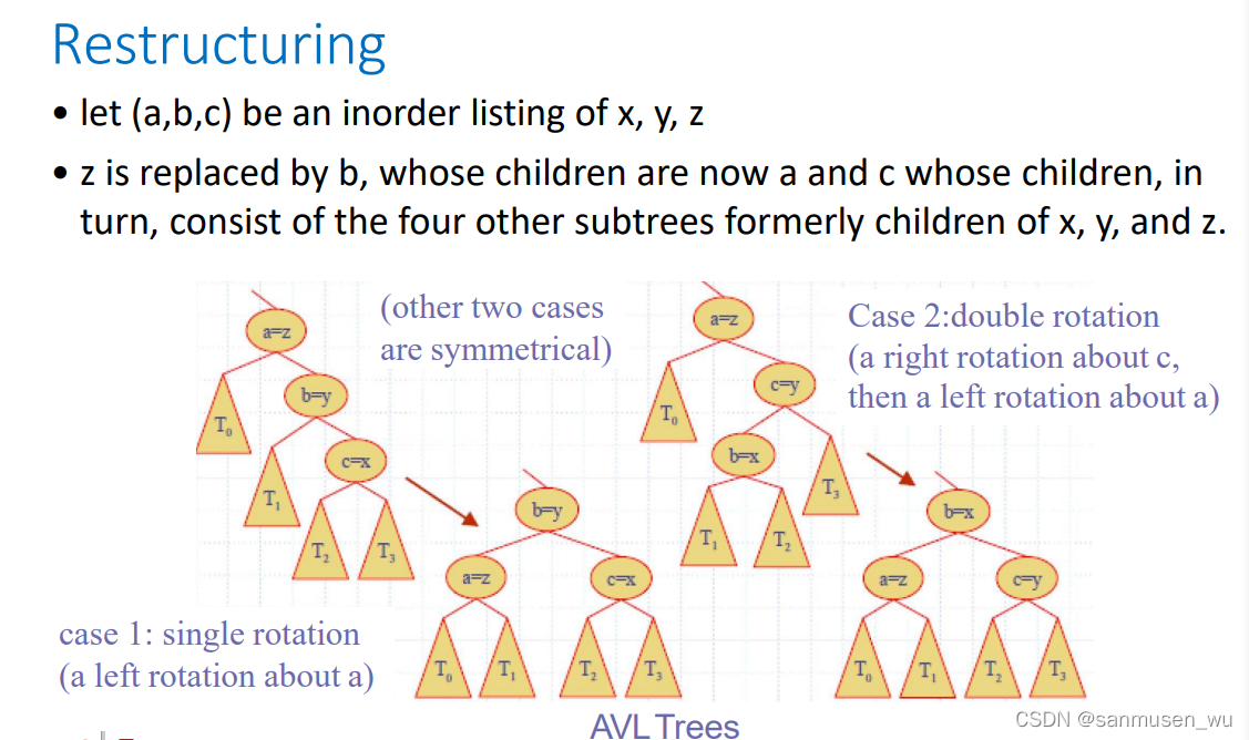
根据中序遍历顺序将x,y,z重命名为（a,b,c），将abc称为三个关键节点
把指向z的指针移到指向b，随后重排abc的四个其他四个子树（依旧保留中序顺序）。
既重排使得b是ac的父节点，abc的子树T₀,T₁…等的中序遍历顺序不变。

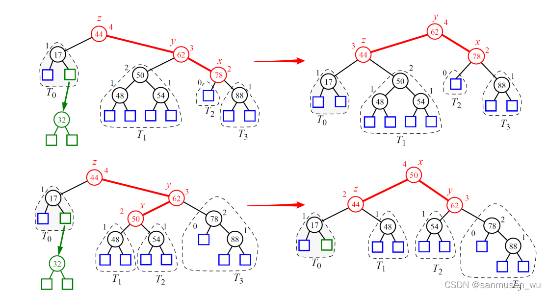
AVL
左旋/右旋既把指向自己的指针移向自己的子关键节点，其中，如果右子节点是关键节点，则本节点向左旋转，将指向自己的指针转而指向右子节点，称为左旋。反之亦然。
左边的情况：a左旋
右边的情况：c右旋，随后a左旋

Algorithm restructure(x):
• Input: A node x of a binary search tree T that has both a parent y and a
grandparent z
• Output: Tree T after a trinode restructuring (which corresponds to a
single or double rotation) involving nodes x, y, and z
• 1: Let (a,b,c) be a left-to-right (inorder) listing of the nodes x, y, and z, and let (T0, T1, T2, T3) be a left-to-right (inorder) listing of the four subtrees of x, y, and z not rooted at x, y, or z.
• 2: Replace the subtree rooted at z with a new subtree rooted at b.
• 3: Let a be the left child of b and let T0 and T1 be the left and right subtrees of a, respectively.
• 4: Let c be the right child of b and let T2 and T3 be the left and right subtrees of c, respectively.

删除AVL tree的节点

找到预删除节点删除，随后重组使得树平衡

增删查改AVL的节点的复杂度都是log(n)

Multi-Way Search Tree

多向搜索树，对于每个节点，都有最少两个子节点，假设d为子节点数量，其节点本身能存储d-1个key-item。
其中又符合：对于任意存储了 ’key k₁, k₂…k_d-1‘ 和 ‘子节点v₁, v₂…v_d’ 的节点

1. v₁所在子树的keys小于k₁
2. v_i所在子树的keys在k_i-1和k_i之间
3. v_d所在子树的keys比k_d-1大

叶子节点不存储item，只作为占位符（也可以存item，但是课件里讨论的都是作为占位符

中序遍历

查找
类似于BST，判断预查找值与keys的大小，选择分支继续查找

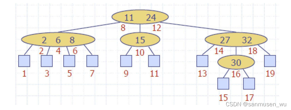
（2，4）trees

Node-Size Property: every internal node has at most four children
Depth Property: all the external nodes have the same depth

根据children数量，其内部节点又被称为2-node,3-node,4-node.

证明（2，4）trees深度为O(logn)
Let n be the height of a (2,4) tree with n items
Since there are at least 2^𝑖 items at depth i = 0, …, h-1 and no items at depth, h, we have
𝑛≥ 1 + 2 + 4 + ⋯ + 2^ℎ−1 = 2^ℎ −1^

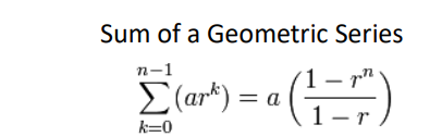
Thus, ℎ ≤ log(𝑛+1)

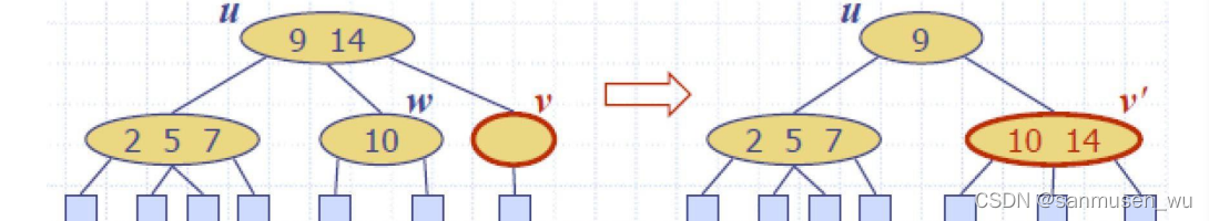
插入操作可能会导致溢出overflow
需要进行切割（split）：

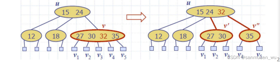
例如v溢出，将32提升到其父节点，并将27，30与35切割成两个子节点，v3划分到【27，30】，v4划分到【35】，溢出可能又提到了父节点，父节点可能也得切割，到根节点可能得从根节点内提一个key作为新的根节点

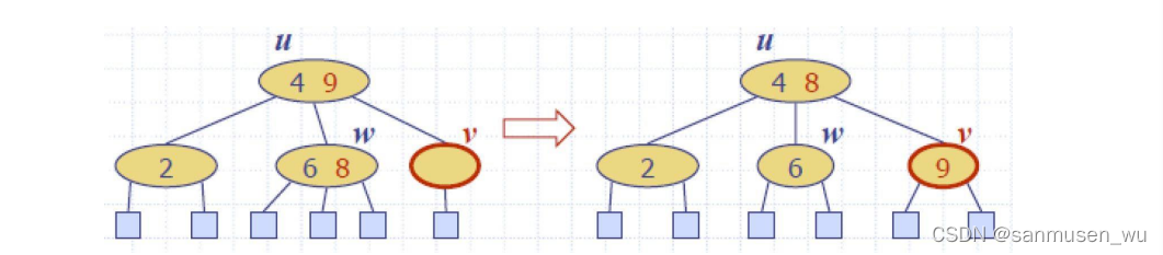
删除操作依旧以提升的方式：例如删除24，类似于BST删除，将24的右子树中的最小值提到24所在位置(inorder successor)，可能会造成underflow，需要fusion或transfer

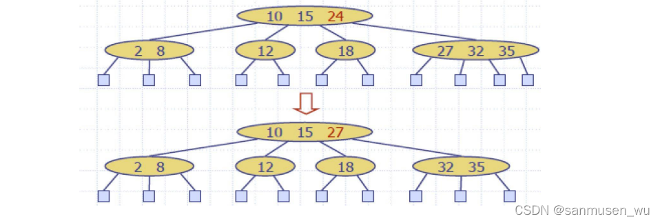
情况一，v节点空了，相邻节点w是个2-node：从u里把14下降并融合w和v及其子节点（父节点可能又underflow了）

情况二，v节点空了，相邻节点是个3-node或4-node：将w的最右子节点移到v，同时8转移到9，9转移到v（有点像右旋-上补右下，下补上

week05

1. 排序结构

1.1. Priority Queues优先级队列

优先级队列类似于先进先出队列，只是每次从队列中取出的是具有最高优先权的元素

1. insertItem(k,e): insert element e having key k into PQ.
2. removeMin(): remove minimum element.
3. minElement(): return minimum element.
4. minKey(): return key of minimum element.

使用优先级队列进行排序：

1. First phase: Put elements of C into an initially empty priority queue, P, by a series of n insertItem operations.
2. Second phase: Extract the elements from P in non-decreasing order using a series of n removeMin operations.

1.2. Heap Data Structure堆

堆是优先级队列的一种实现，分为大根堆/小根堆：对于任意节点，其左右子树的值都小于/大于该节点的值。
max-heap根元素最大
min-heap根元素最小
插入删除操作都是对数级insertions and deletions to be performed in logarithmic time

1. a binary tree T is full if each node is either a leaf or possesses exactly two child nodes.
2. A complete binary tree of height h is a binary tree which contains exactly 2^d nodes at depth d, 0 ≤ d ≤ h.
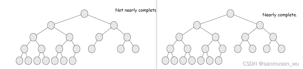
3. A nearly complete binary tree of height h is a binary tree of height h in which:
   1. a) There are 2^d nodes at depth d for d = 1,2,…,h−1,
   2. b) The nodes at depth h are as far left as possible.
      .

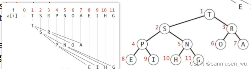
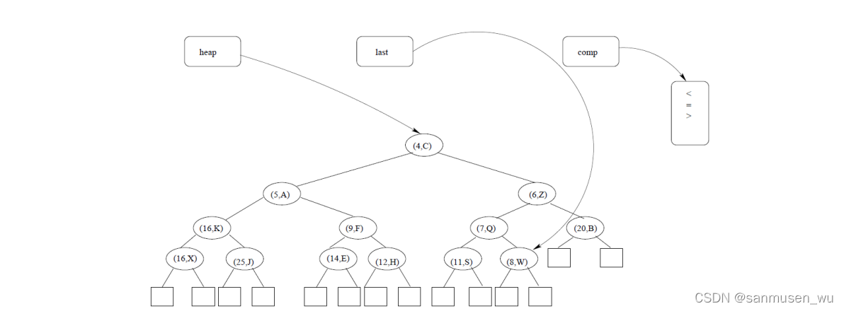
对于complete的树，可以使用数组存储，其下标0存储根节点，下标1开始存储有值的节点

For any given node at position i:
•Its Left Child is at [2i] if available.
•Its Right Child is at [2i+1] if available.
•Its Parent Node is at[ ⌊i/2⌋ ] if available.

因为这里有根节点，所以这里寻址与之前的BST有点不一样

除了heap本身外，还需要存储last指针，指向数组中最后一个堆元素，以及comp定义了比较方法

Theorem: A heap storing 𝑛 keys has height 𝑶(log𝑛)

Proof: (we apply the complete binary tree property)
Let h be the height of a heap storing 𝑛 keys
Since there are 2^𝑖 keys at depth 𝑖 = 0,… , ℎ − 2 and at least one key at depth ℎ − 1, we have n ≥ 1 + 2 + 4 + ⋯ + 2^ℎ−2 + 1
Thus, n ≥ 2 ^ℎ−1, i.e., ℎ ≤ log 𝑛 + 1

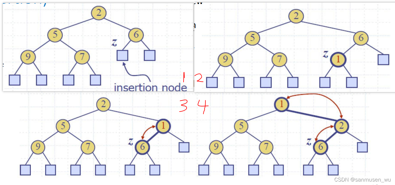
插入 Up-heap bubbling (insertion)

插入一个新元素到尾部后，需要往上重排

1. Find the insertion node 𝑧 (the newlast node)
2. Store 𝑘 at 𝑧 and expand 𝑧 into an internal node
3. Restore the heap-order property：
   1. After the insertion of a new key 𝑘, the heap-order property may be violated
   2. Algorithm upheap restores the heap-order property by swapping 𝑘 along an upward path from the insertion node
   3. Upheap terminates when the key 𝑘 reaches the root or a node whose parent has a key smaller than or equal to 𝑘
   4. Since a heap has height 𝑂(log 𝑛), upheap runs in 𝑂(log 𝑛)time

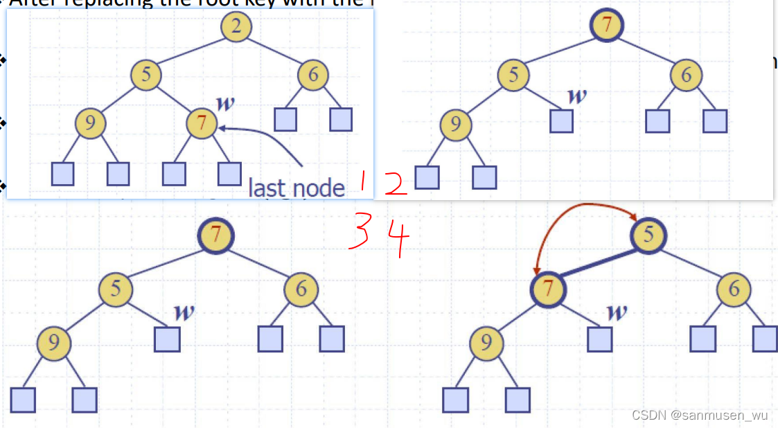
删除 Down-heap bubbling (removal of top element)

取出即为删除，且只能取堆顶（也就是最大/最小的值），取之后需要把尾提上来然后往下重排

1. Replace the root key with the key of the last node 𝑤
2. Compress 𝑤 and its children into a leaf
3. Restore the heap-order property：
   1. After replacing the root key with the key 𝑘 of the last node, the heap-order property may be violated
   2. Algorithm downheap restores the heap-order property by swapping key 𝑘 along a downward path from the root
   3. Upheap terminates when key k reaches a leaf or a node whose children have keys greater than or equal to 𝑘
   4. Since a heap has height 𝑂(log 𝑛), downheap runs in 𝑂(log 𝑛)time

2. 排序算法

归并排序MergeSort
先分成左右两部分，然后递归调用O(logn)使得左右两部分有序，然后O(n)把左右两有序部分合起来成一个总体有序。
平均复杂度O(nlogn)
INT102 week03

快速排序QuickSort
快速排序也用到了分治的思想
算法如下：

1. 从左端点到右端点之间随机挑选一个元素，
2. 将小于这个元素的放这个元素左边L，大于这个元素的放这个元素右边R
3. 分别排序L和R区域
   平均复杂度：O(nlogn)
   最差：每次挑选的都是区域内最大/最小值-O(n²）

week06

Divide and Conquer

• Divide: If the input size is small then solve directly, otherwise divide the input data into two or more disjoint subsets.
• Recur: Recursively solve the sub-problems associated with the subsets.
• Conquer: Take the solutions to the sub-problems and merge them into a solution to the original problem

Running time

先给出分治的等式：

       b               if n<2
T(n)={
       2T(n/2)+bn      otherwise

Master Method

将上式抽象为如下形式

       c               if n<d
T(n)={
       aT(n/b)+f(n)    otherwise
where d>=1,a>0,c>0,b>1

则对应的T(n)的时间复杂度有三种情况:
(此处 logb(a)=log_ba，编辑器打不出来)

1. Case 1：if f(n)=O(n^logb(a)-ε) for some constant ε>0, then T(n)=θ(n^logb(a))
2. Case 2：if f(n)=θ(n^logb(a)) , then T(n)=θ(n^logb(a)logn)
3. Case 3：if f(n)=Ω(n^logb(a)+ε) for some constant ε>0, and if af(n/b) <= cf(n) for some constant c<1 and all sufficiently large n, then T(n)=θ(f(n))

判断是哪个case只需比较f(n)和n^logb(a)幂指数大小关系

1. Case 1: applies where f (n) is polynomially smaller than the special function n^logb(a).
2. Case 2: applies where f (n) is asymptotically close to the special function n^logb(a).
3. Case 3: applies where f (n) is polynomially larger than the special function n^logb(a).

*f(n) is polynomially smaller than g(n) if f(n)=O(g(n)/n^ϵ) for some ϵ>0.
*f(n) is polynomially larger than g(n) if f(n)=Ω(g(n)n^ϵ) for some ϵ>0

例子1：
考虑如下式子：
T(n)=4T(n/2)+n
a=4,b=2,f(n)=n
n^logb(a)=n², f(n)为一次项 < nlogb(a)为二次项
使用case1，f(n)=O(n^2-ε) for ε=1
所以T(n)=θ(n^logb(a))=θ(n²)

例子2：
T(n)=T(2n/3)+1
a=1,b=3/2,f(n)=1
n^logb(a)=1, f(n)为常数项 = n^logb(a)为常数项
使用case2，f(n)=θ(n^logb(a))
所以T(n)=θ(n^logb(a)logn)=θ(logn)

例子3：
T(n)=T(n/3)+n
a=1,b=3,f(n)=n
n^logb(a)=n⁰=1, f(n)为一次项 > n^logb(a)
使用case3，f(n)=Ω(n^logb(a)+ε)=Ω(n^0+ε) for ε=1,
所以T(n)=θ(f(n))=θ(n)

例子4：
T(n)=2T(n/2)+nlogn
a=2,b=2,f(n)=nlogn
n^logb(a)=n¹=n, f(n)为nlogn，此处需要注意nlogn与n不是多项式大于（polynomically larger）的关系，应当是渐进（asymptotically less）小于，f(n)/n^logb(a)=(nlogn)/n=logn，logn对于任意非负数c，都要渐进小于n^c。所以情况落于case2与case3之间

(如何求解像T(n)=2T(n／2)+nlgn这种递归式? - Iterator的回答 - 知乎
https://www.zhihu.com/question/37097499/answer/1906449615)

例子5：
T(n)=2T(n^1/2)+logn
这种形式不能使用master method，需要代换和变形
先用k代换logn, k=logn,n=2^k,
T(n)=T(2^k)=2T(2^k/2)+k
将函数T(2^k)变形为T₁(k)，与上面的代换不同，这里k的值没有发生变化
T₁(k)=2T₁(k/2)+k
对T₁使用master method可以得知T₁(k)=O(klogk)
套回代换k=logn, 得T(n)=O(lognloglogn)

Matrix Multiplication

问题描述： 假设现有个nxn的矩阵X和Y，我们想要计算它们的积Z=XY，

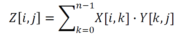
爆算是O(n³):

n=A.rows
let C be a new nxn matrix
for i=1 to n
	for j=1 to n
		cij=0
		for k=1 to n
			cij=cij+aik*bkj
return C

Divide-and-conquer algorithm O(n³):
Suppose n is a power of two and let us partition X, Y, and Z each into four (n/2)×(n/2) matrices, so that we can rewrite Z = XY as

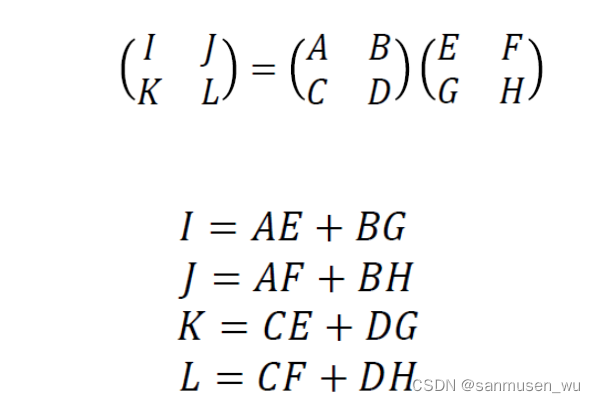
By the above equations, we can compute 𝐼, 𝐽, 𝐾, and 𝐿 from the eight recursively computed matrix products on (n/2)×(n/2) subarrays, plus four additions that can be done in 𝑂(𝑛²)time.

T(n)=8T(n/2)=bn² —for some constant b > 0
This equation implies: T(n) = 𝑂(𝑛³) by the master theorem

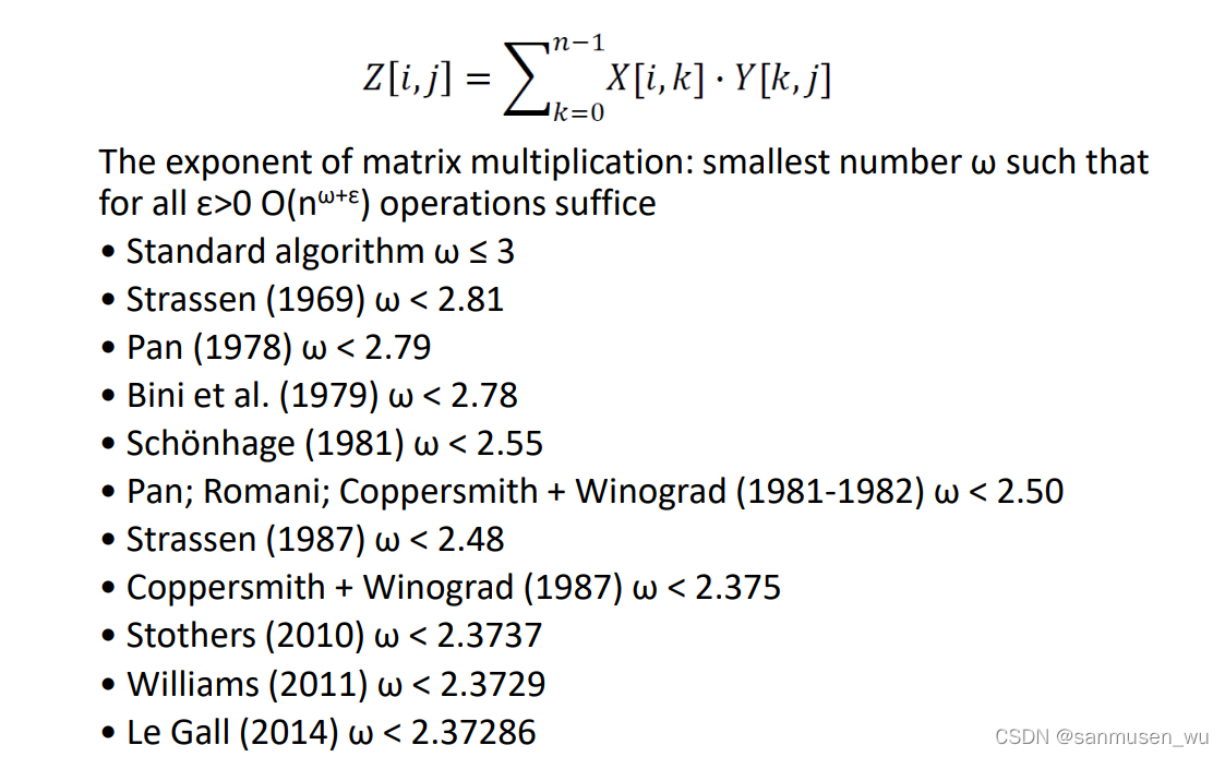
Strassen’s algorithm 𝑂(𝑛^log7):
involving the subarrays 𝐴through 𝐺 so that we can compute 𝐼, 𝐽, 𝐾,and L using just seven recursive matrix multiplications (by Volker Strassen 1969).

Define seven submatrix products:

S₁=A(F-H)
S₂=(A+B)H
S₃=(C+D)E
S₄=D(G+E)
S₅=(A+D)(E+H)
S₆=(D-E)(G+H)
S₇=(A-C)(E+F)

Given these seven submatrix products, we can compute 𝐼, 𝐽, 𝐾,and L as:

I=S₅+S₆+S₄-S₂=AE+BG
J=S₁+S₂=AF+BH
K=S₃+S₄=CE+DG
L=S₁-S₇-S₃+S₅=CF+DH

Thus, we can compute 𝑍 = X𝑌 using seven recursive multiplications of matrices of size (n/2)×(n/2). Thus, we characterize the running time 𝑇(𝑛) as:

T(n)=7T(n/2)+bn²—for some constant 𝑏 > 0.
By the master theorem, we can multiply two n x n matrices in 𝑂(𝑛^log7)time using Strassen’s algorithm.

Ranking system

比如说豆瓣给电影打分，你的账户对十个电影的打分是
1 2 3 4 5 6 7 8 9 10
另外两个人对这十个电影的打分是
2 7 10 4 6 1 3 9 8 5
8 9 10 1 3 4 2 5 6 7
如何评判这两个人谁和你的观影口味更相近。

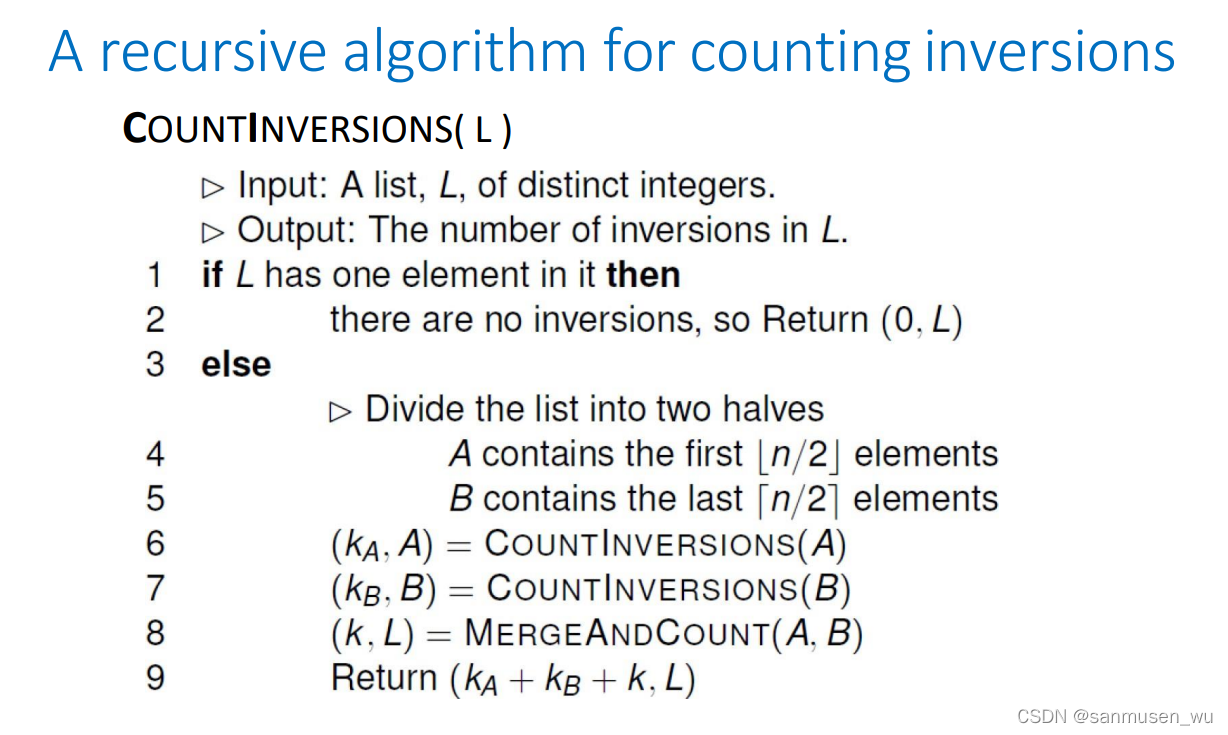
方法一：count the number of inversions：
inversion: in a₁,a₂,a₃,a₄, if i < j, then a_i > a_j
In other words, to find the number of inversions, we count the pairs i ≠ j that are out of order in the permutation

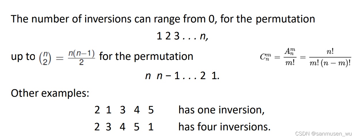
example:
2 1 3 4 5 has one inversion,
2 3 4 5 1 has four inversions.

So how do we count the number of inversions in a given permutation of n numbers?
The “naive” approach is to check all pairs to see if they form an inversion in the permutation. This gives an algorithm with O(n²) running time.

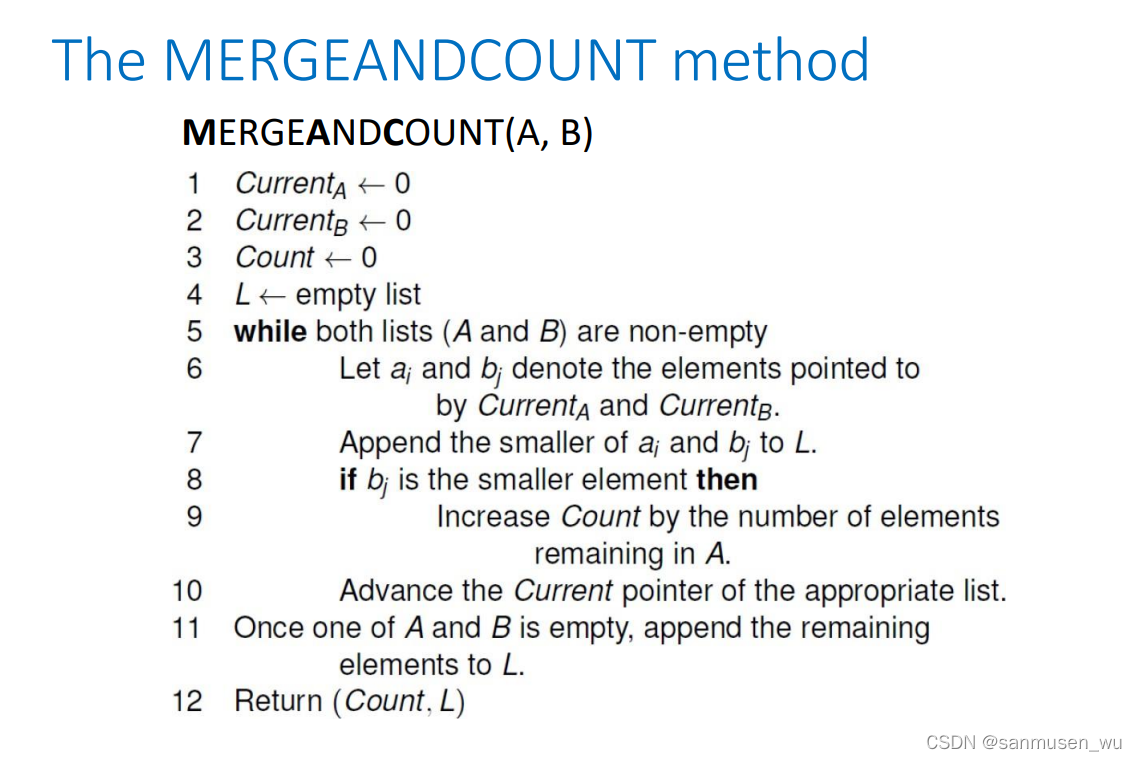
We can count inversions using a divide-and-conquer algorithm that runs in time O(n log n).—performing a modified MergeSort!

In terms of the ranking system describe earlier, the number of inversions for a permutation is a measure of how “out of order” it is as compared to the identity permutation
1 2 3 . . . n
and hence could be used to measure the “similarity” to the identity permutation.

week08

1. 背包优化问题 Optimize Problem

Knapsack Problem背包问题
n个物品，每个物品都有重量w和价值b，现有一负重不超过W的背包，要求挑选物品放进背包使得他们的总价值最大
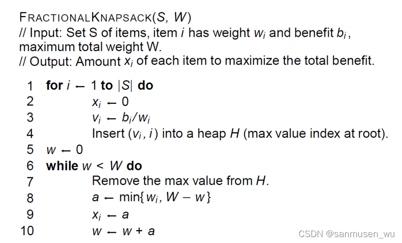
Fractional Knapsack Problem （FKP）：
部分背包问题
在背包问题的基础上，可以将商品的一部分装入，重量和价值也是一部分

1.1. Greedy Method 背包问题-贪心算法

贪心算法思路简单，每步都选择当前局部最优解，但无法保证得到全局最优解

背包问题-贪心：
在不超过限重的情况下，先后挑选最贵的放入，估值函数(b)
或者先挑最轻的放入

部分背包问题-贪心：
在不超过限重的情况下，先后挑选单位价值最大的尽可能放入，估值函数(b/w)，时间复杂度O(nlogn)

x_i：拿取一个物品的部分重量，0 < x_i < w_i
背包内的物品总价值：b_i*x₁/w_i

Try this out: (2, 2) ,(3, 7),(4, 9),(5, 9) for a maximum weight of 6.

(w,b)	(2, 2)	(3, 7)	(4, 9)	(5, 9)
Value index	1	2.33	2.25	1.8
Selection xi	0	3	3	0

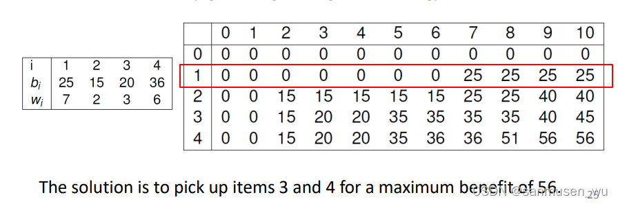
1.2. Dynamic Programming背包问题-动态规划

ref:动态规划
动态规划自底向上，解决子问题后，解决总问题。
Basic Idea：Solve bottom-up, building a table of solved subproblems that are used to solve larger ones

n个物品，重量w和价值b
B[k,w]:当前背包内考虑了前k（0<k<n)个物品，剩余容量为w，此时背包的总价值。
每次背包都会逐个考虑下标为k的物品，考虑拿与不拿标号为k的物品

B[0,w]=0
		/ B[k-1,w]						if w<wk
B[k,w]=
		\ max( B[k-1,w], bk+B[k-1,w-wk] )

example：
限重W=10，
一次dp为红框框所示

2. 单线程区间调度问题 Interval Scheduling Problem

给定n个tasks，每个task都有开始时间s_i，结束时间f_j，task不能同时进行。求限定时间T内，如何选择tasks使得尽可能多的tasks被完成。

2.1. 区间调度-贪心算法

挑选开始时间最早的：
for example, we always pick the first available task with the earliest start time
估值函数（s_i)

Counter-example：
如果最早到的task直接占据所有时间：

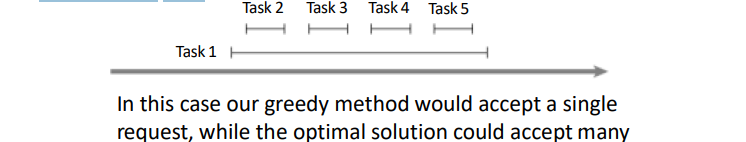
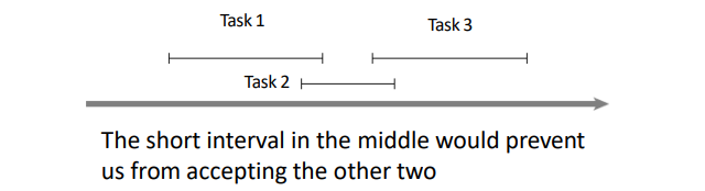
挑选持续时长最短的
for example, we always pick the "short“ intervals first，估值函数 -(f_i-s_i)

Counter-example：

挑选结束时间最早的 (贪心中比较靠谱的
we always accepting the task that finishes first.估值函数 -(f_i)

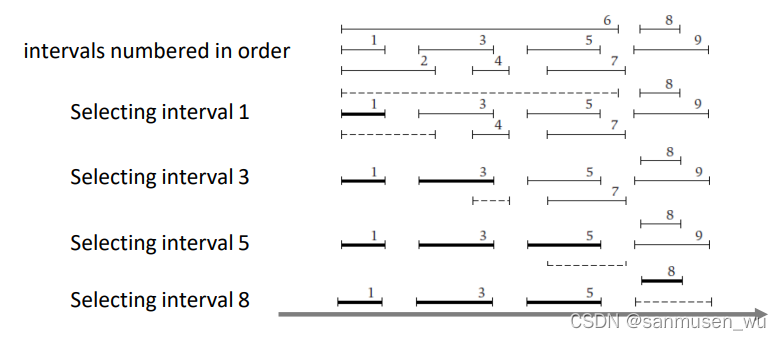
细线表示可选，粗线表示选定，虚线表示与已选的冲突

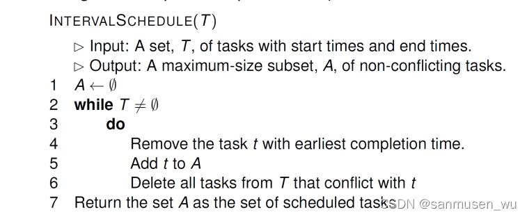
Order the tasks in terms of their completion times. Then select the task that finishes first, remove all tasks that conflict with this one, and repeat until done.
按照结束时间排序，然后挑选
时间复杂度：O(nlogn) (the main time will lie in sorting the tasks by their completion times).

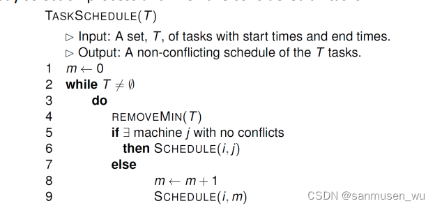
3. 多线程区间调度问题 Task Scheduling

依旧是n个tasks，task有开始时间s结束时间f，task可以同时在不同的线程中运行，求完成所有tasks所需的最少线程数量

3.1. 多线程区间调度-贪心算法

1. This time we consider the tasks ordered by their start times.
2. Then for each task i, if we have the machine that can handle task i, it is scheduled on that machine.
3. Otherwise, we allocate a new machine, schedule task i on it, and repeat the greedy selection process until we have considered all tasks in T

3. Graph 图

3.1. 图的介绍

node=vertice=set V
edge=pair-wise connection=set E

graph=(V,E)
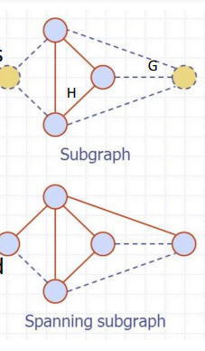
subgraph=(V₁,E₁), V₁∈V，E₁∈E
spanning subgraph=(V,E₁), E₁∈E

path=sequence of alternating vertice and edges
simple path=path such that all its vertices and edges are distinct

tree=undirected，connected，no cycle graph
spanning tree= tree (subgraph) of a graph, not unique
forest=undirected，no cycle graph
spanning forest= forest (spanning subgraphs) of a graph

边分为有向边(directed edge, (u,v)代表从u到v) 和 无向边(undirect edge)
一条边连着的两个点称为end vertices of this edge，这两个点相邻adjacent
一个点连着的多条边称为edges incident on a vertex，这些边的数量称为degree of this vertex

图分为有向图(Directed graph)和无向图(Undirect graph)
所有点之间都有边的图称为connected graph，如果图G不完全连通，则其最大的可连通的子图被称为connect components
有环图cyclic graph
无环图acyclic graph，有向无环图directed acyclic graphs（DAG）
假设图的边数量为m，点数量为n，连通图m>=n-1，树m=n-1，森林m<=n-1

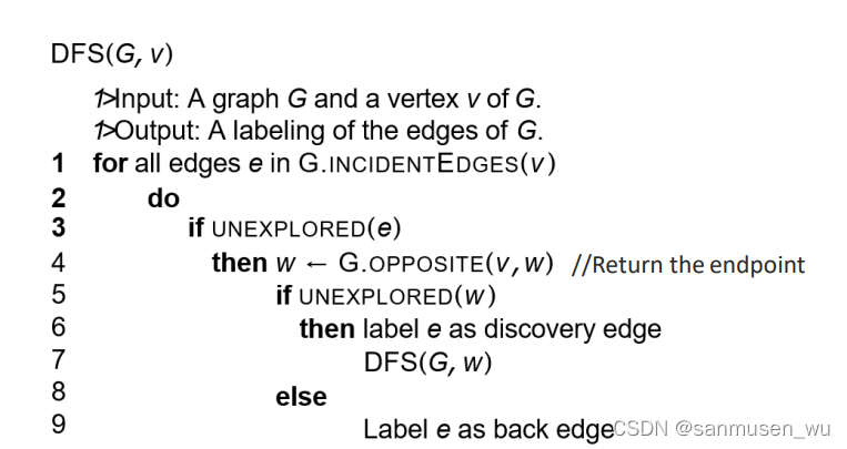
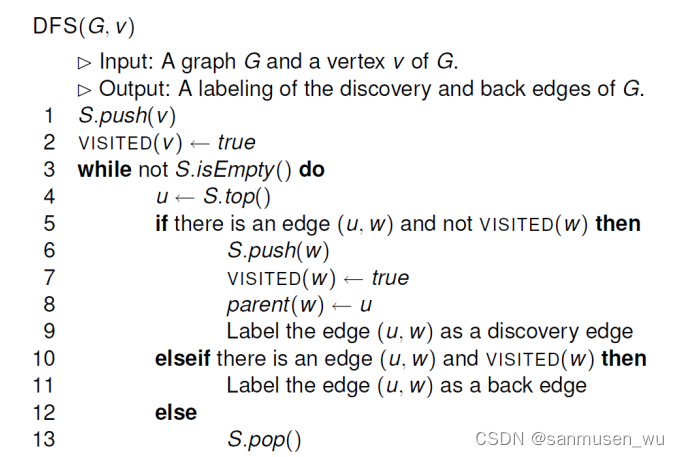
3.2. 图的遍历

DFS：深度优先deep first
可以用来做生成树Produces a spanning tree, such that, all non-tree edges are back edges.
Back edge: It is an edge (u, v) such that v is ancestor of node u but not part of DFS tree.

非递归版本

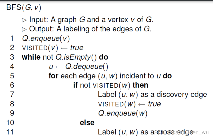
BFS：广度优先Breadth first
可以用来寻找最短路径
也能用来做生成树Produces a spanning tree, such that, all non-tree edges are cross edges.
Cross edge：It is a edge which connects two nodes such that they do not
have any ancestor and a descendant relationship between them.

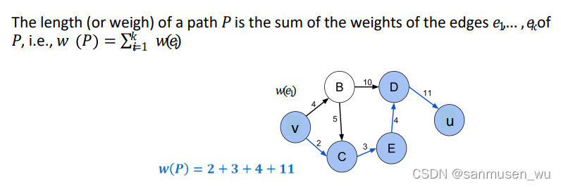
3.3. Weighted Graph带权图

权重边
P: v->c->e->d->u

Single-Source Shortest Paths
For some fixed vertex 𝑣, find the shortest path from 𝑣 to all other vertices 𝑢 ≠ 𝑣 in 𝐺 (viewing weights on edges as distances)

要求边权值非负
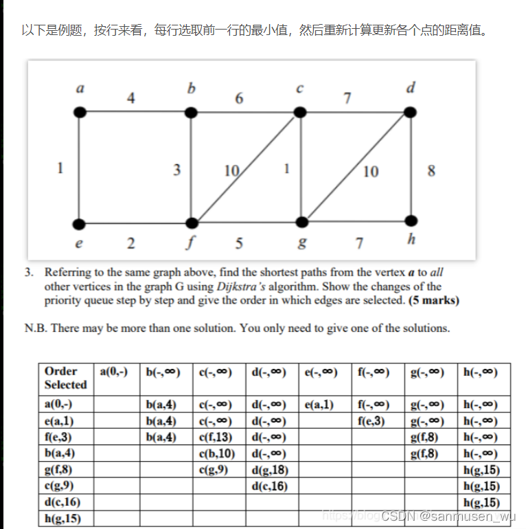
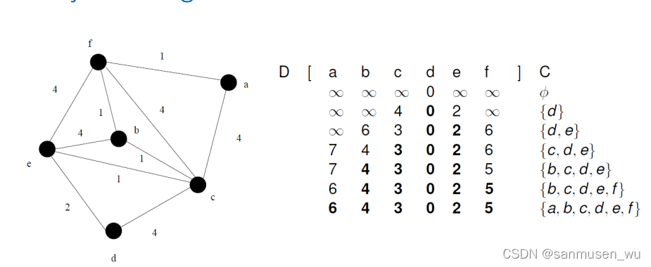
Dijkstra’s algorithm

边的松弛Edge Relaxation：
D(z)表示源点到z的距离，如果找到了使D(z)更小的路径，则更新D(z)

dijkstra算法能够用上次确定的点松弛未确定的点，从而得到未确定的点中的最小值并将他变为确定的点，继续进行松弛。详情见上面链接

当边权值可负数，且边为有向边时
Bellman-Ford

边的松弛Edge Relaxation：
it does not use it with the greedy method. Instead it performs a relaxation of every edge exactly (V − 1) times.
This relies on the fact that, if there are no negative cycles, then there is a shortest path from v to any other vertex in G with at most V − 1 edges.

Bellman-Ford算法个人理解为广度优先的查找，可以认为它在逐渐把距离源点一条边的那些点，距离源点两条边的那些点，距离源点三条边的那些点…逐个松弛一遍。当松弛V-1次时，如果无环的话，所有点应该都是最短状态了。

week09

1. Minimum Spanning Tree最小生成树

什么是最小生成树：G是一个带权无向图，找到使总边权最小的生成树T（无环子生成图）

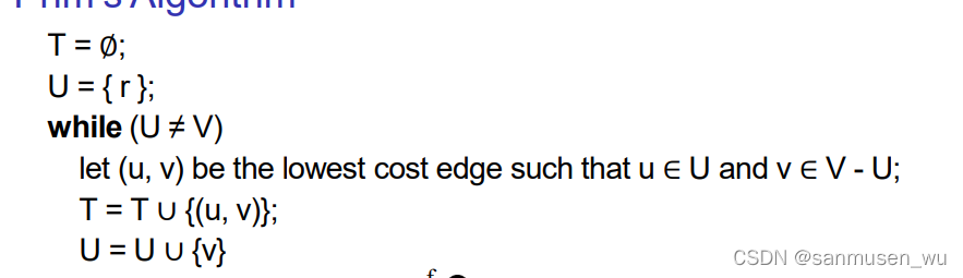
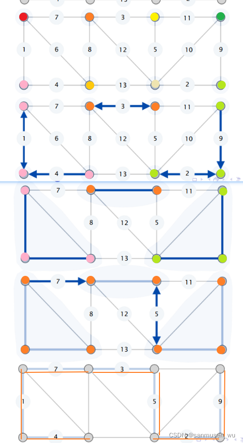
1.1. Prim’s Algorithm

INT102 Prim’s Algorithm
假设一个一开始只包含根节点的簇U，从根节点开始，依次选择【邻近簇U内的点，位于簇U外，距离簇U最短】的点加入簇U。直到所有点都包含在簇内.

1.2. Kruskal’s Algorithm

INT102 Kruskal’s Algorithm
假设一个一开始为空的簇，所有边从小到大排序，依次选择【不会造成环】的边加入簇。直到所有点都包含在簇内。

1.3. Borůvka’s algorithm

一开始将图中的每个点都看成一个簇。
重复每轮迭代，直到所有点都在生成树内：

1. 对于每个簇，考虑与簇相连的最短的边，如果该边不在生成树内，则将这条边加入生成树。并将该边相连的两个簇合并。

2. Flow Network

2.1. flow 流

网络流包含：

1. A weighted graph G with nonnegative integer edge weights，边e的权重也可被称为e的容量(capacity) c(e)
2. Two distinguished vertices, s and t of G, called the source and sink. s只有指向外的箭头，t没有指向外的箭头

流的特性：

1. 任意一条线e上的流 f(e) 不能超过其容量c(e)
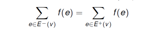
   0<=f(e)<=c(e)
2. 除了s和t，其他节点v的 入流总和 等于 出流总和，既中间节点不能消耗流量。
   
3. 网络流（a flow for a network) 的总和为source节点出流的总和 或 sink节点入流的总和，称为|f|或value of a flow

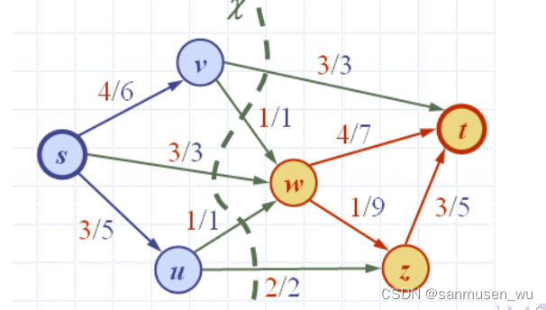
2.2. Cut 割

将点集分成两部分S和T，s属于S，t属于T，称为割X。
forward edge of cut： 从S指向T
backward edge of cut: 从T指向S

Flow f(x) across cut X: total flow of forward edges minus total flow of backwardedges.S的出流减去S的入流，称为通过割{S,T}的流量
Capacity c(x) of cut X: total capacity of forward edges S的出流的容量
Minimun cut：使c(x)最小的割

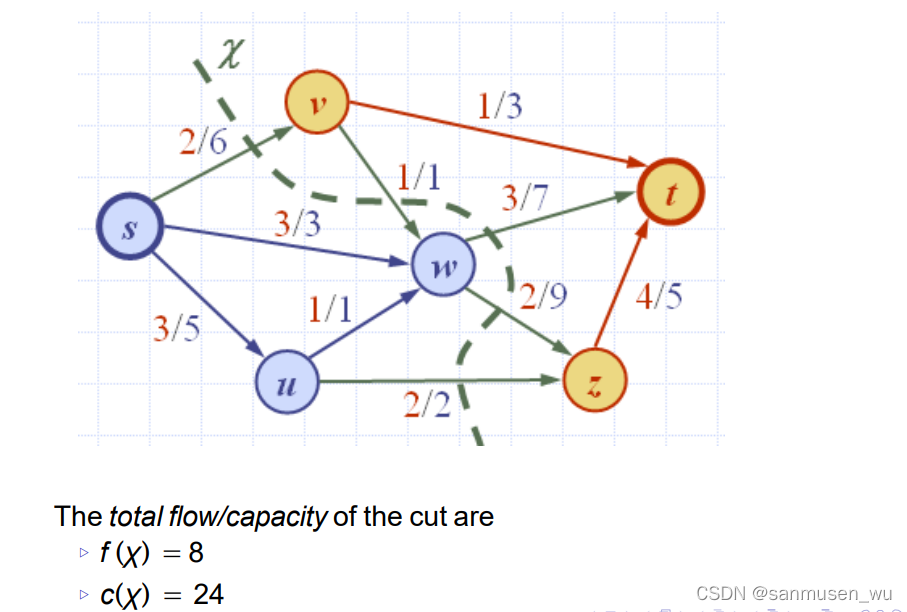
Lemma 1: 对于任意割X，f(X)=|f|
Lemma 2: 对于任意割X，f(X)<=c(X)

Theorem 1： The value of any flow is less than or equal to the capacity of any cut, i.e., for any flow f and any cut χ,we have |f | ≤ c(χ).

2.3. Augmenting Path增广路径

残差容量Residual capacity:
Let e be an edge from u to v

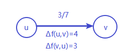
1. Residual capacity of e from u to v: ∆f(u,v) = c(e) − f(e)，顺着箭头看的话残差容量为 容量减去现有流量，既还可以增加多少流量。
2. Residual capacity of e from v to u: ∆f(v,u) = f(e)，反着箭头的话直接是现有流量。

对于一个从s到t的不经过重复点的路径π，该路径的残差容量/瓶颈容量（bottleneck capacity，∆f (π) ）为路径上的每个边的残差容量的最小值
如果该最小值>0，则称该路径为增广路径。

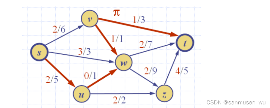
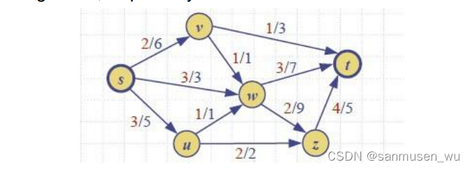
|f|=7
∆f(s,u) = 3, ∆f(u,w) = 1, ∆f(w,v) = 1, ∆f(v,t) = 2.
∆f (π) = 1

不难发现该路径上的流量可以+1，使得流的总流量增加1.
∆f(s,u) = 3-1=2, ∆f(u,w) = 1-1=0, ∆f(w,v) = 1-1=0, ∆f(v,t) = 2-1=1.

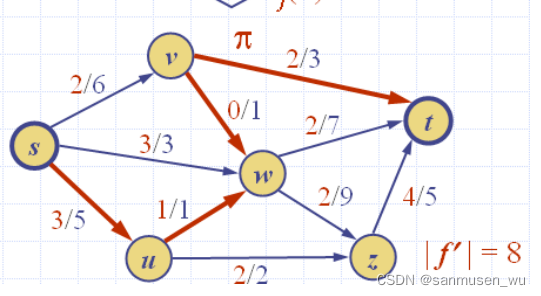
特别注意w，发现路径沿着u->w->v方向但是（v，w）箭头指向w，这就是上文残差容量定义的巧妙之处：
顺着路径将沿路径方向的箭头流量+∆f (π) ，如果箭头逆路径则流量-∆f (π) ，可以使得

1. 顺路径的节点（如u）入流量增大∆f (π)，且出流量增大∆f (π)，扩增发生在u。
2. 逆路径的节点（如w）的入流量增大∆f (π)的同时减小∆f (π)，出流量保持不变，经过w本身的流量不变，而扩增发生在路径方向上w的上一个节点u（v到w流量的减小使得u到w的流量可以增加）。

Lemma 3： Let π be an augmenting path for flow f in network N. There exists a flow f’ for N of value |f’| = |f| + ∆f(π)

2.4. 最大流问题Maximum Flow

对于一个给定的网络，如何分配各个边的流量，使网络流的流总和最大。

发生如下情况，则称当前网络流最大：

1. Lemma 4： If a network N does not have an augmenting path with respect to a flow f, then f is a maximum flow. Also, there is a cut χ of N such that |f| = c(χ). 没有扩增路径。
2. Theorem 2: The value of a maximum flow is equal to the capacity of a mimimumcut. 最大流等于最小割。

Max-Flow and Min-Cut:
Define

• ▷ Vs set of vertices reachable from s by augmenting paths
• ▷ Vt set of remaining vertices

Cut χ = (Vs,Vt) has capacity c(χ) = |f|

• ▷ Forward edge: f (e) =c(e)
• ▷ Backward edge: f (e) =0

Thus, flow f has maximum value and cut χ has minimum
capacity. Below we have c(χ) = |f | =10.

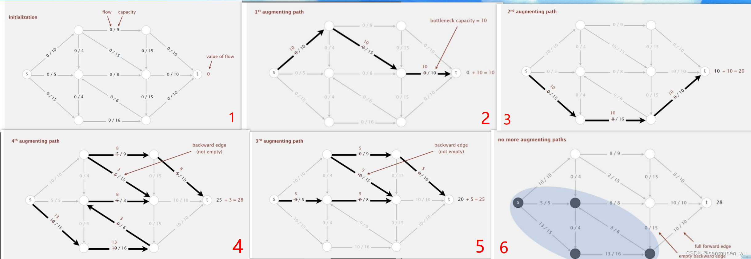
2.4.1. Ford-Fulkerson Algorithm

将所有边的流初始化为0，重复找出增广路径并计算该路径的瓶颈容量并扩增，直到无增广路径。

增广路径可以通过dfs来找，从s开始依次向下寻找残差容量大于0的路径。

ref1

3. Bipartite Matching二分图最大匹配

二分图：graph G = (V,E) is bipartite if and only if

1. The set V can be partitioned into two sets, X and Y .点集被划分为两个集合。
2. Every edge of G has an endpoint in X and the other endpoint in Y.每条边相连的两个点一个在X，一个在Y。既X和Y各自里面没有线连结，X和Y之间可以连线。

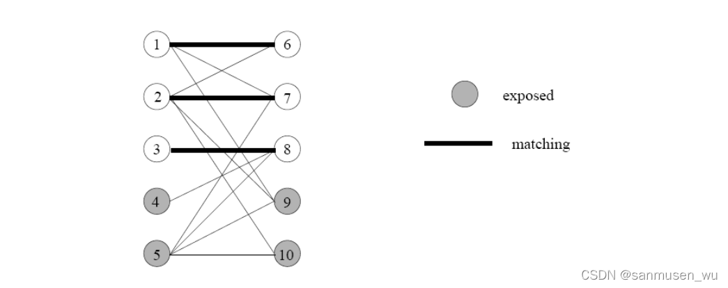
匹配：matching M ⊆ E is a set of edges that have no endpoints in common. Each vertex from one set has at most one “partner” in the other set.匹配是线集的子集，其中每个点最多只能连一条线到对面
如果某个点没有被线连结，则称该点exposed/unmatched
如果没有点未匹配，则称匹配perfect

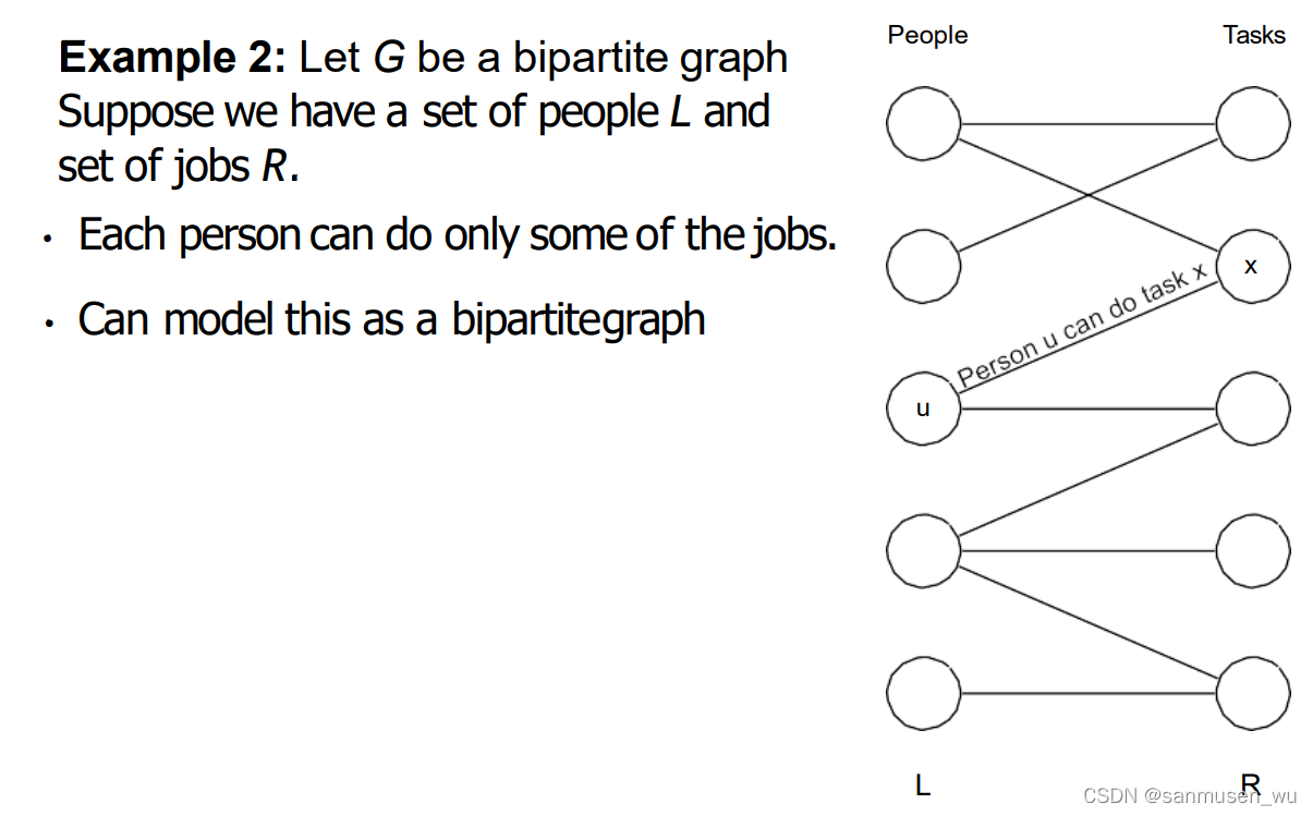
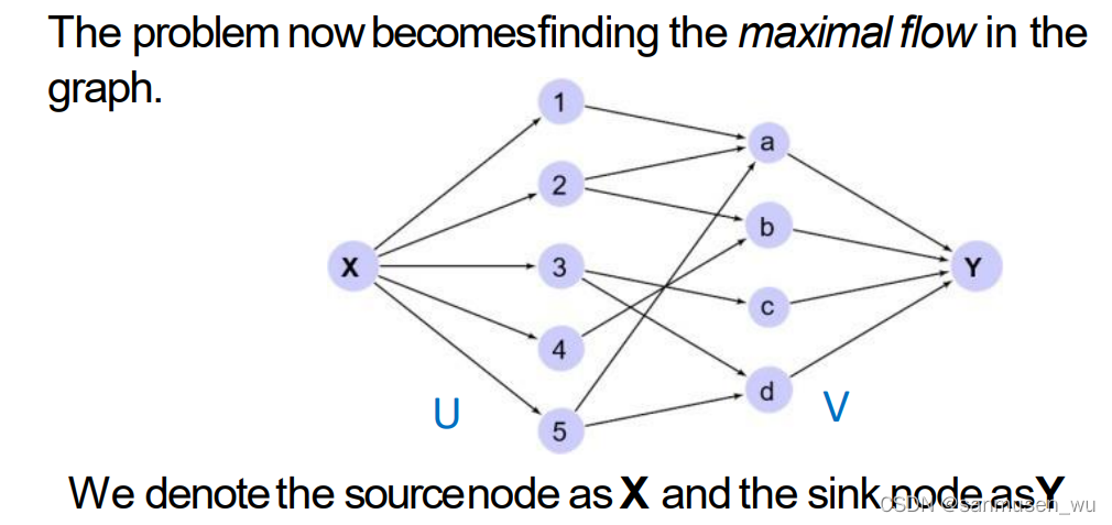
3.1. maximum bipartite matching problem

Given a bipartite graphG = (A ∪ B ,E ), find an S ⊆ A × B that is a
matching and is as large as possible.
既使得左右两个集合之间的匹配连线最大
其中A，B在题干中给出

例题：

3.2. reduce

使用网络流解决二分图最大匹配

在集合U，V两侧分别设置source和sink，并假设流的方向从U到V。
二分图最大匹配问题此时变成了网络流的最大流问题。可以使用边容量为1的Ford–Fulkerson algorithm。

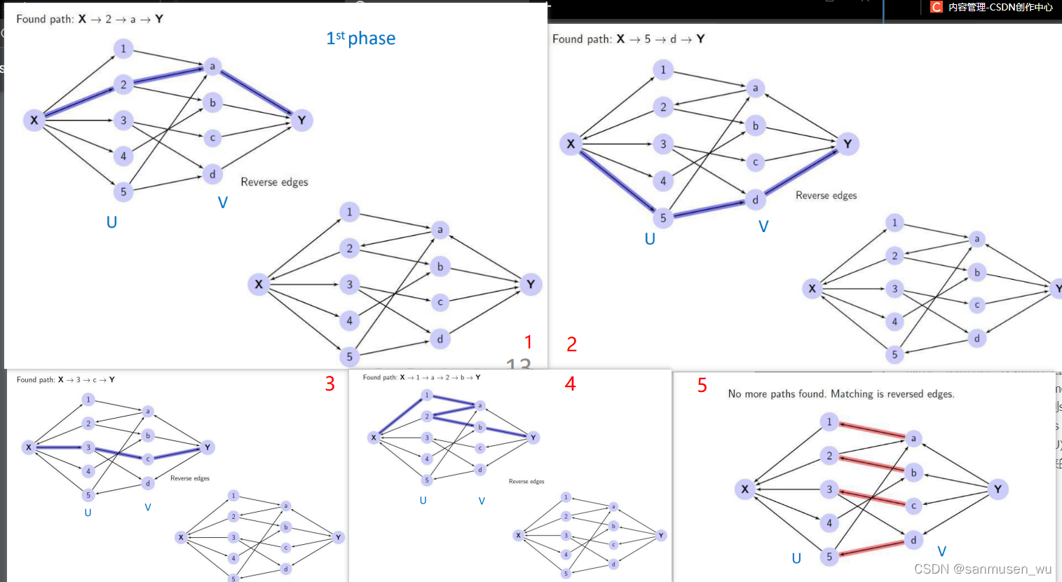
3.3. 匈牙利算法

除了Ford–Fulkerson algorithm，还可以使用相较简单的算法如匈牙利算法，来解决这类无权重有向图问题。区别个人感觉是路径寻找会方便一点，不用考虑路径里有反箭头。

Solving maximal flow for an unweighted directed graph:

1. Construct the directed graph with a source and sink node.
   依旧是添加source和sink点，假设U->V流向
2. Using a search method to find a path from the source to the sink.
   使用路径寻找（dfs，bfs）算法，顺着箭头找到一条从source到sink且不经过重复点的路，既寻找增广路径。
3. Once a path is found, reverse each edge on this path.
   当找到一条路径时，反转路径上的所有箭头（既用取反代表扩增一次）
4. Repeat step2 and 3 until no morepaths from the sink to source exist.
   重复2和3直到没有source到sink的路径
5. The final matching solution is then the set of edges between U andV that arereversed(i.e. run from V to U).
   算法结束时，集合间所有反过来的箭头的集合即为解

证明算法会结束：

每次迭代时路径的最后一条箭头p必指向sink且路径中没有从sink出发的箭头，反转时p被反转，则之后的路径中必不包含p。假设初始一共有n条箭头指向sink，则至多经过n次迭代，算法将终止。

一点理解：

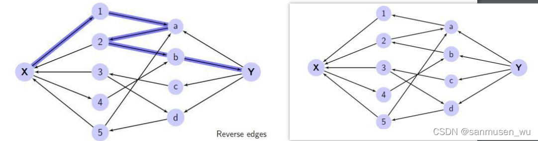
当集合中间出现如上图的z字线路，原本 2<-a 代表2与a配对。
取反后，变成1<-a,2<-b，代表1与a配对，2与b配对。
可以理解为 这次为1尝试分配任务时，发现考虑中的任务a已经被2认领了，此时再去考虑2能不能转去接受其他未认领的任务，发现任务b此时未被认领，于是1和2此时都有任务了，扩增一次。

week10

Toprotect sensitive information, we must ensure the following
goals aremet:

1. Data Integrity: Information should not be altered without detection.
2. Authentication: Agentsinvolved in the communication must be identified.
3. Authorization: Agents operating onsensitive information mustbe authorisedto performthose operations.
4. Nonrepudiation: If binded by contracts, agents cannot drop out of their obligations without being detected.
5. Confidentiality: Sensitive information must be kept secret from agents that are not authorisedto access it.

1. Review

1.1. Set of integers

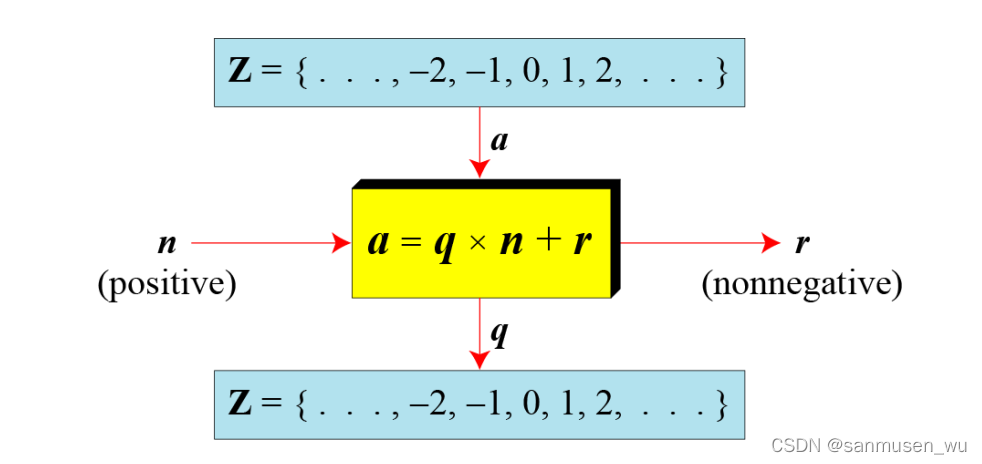
集合内包含整数
Z = {…, -2, -1, 0, 1, 2, …}

1.2. Binary Operations

加减乘操作

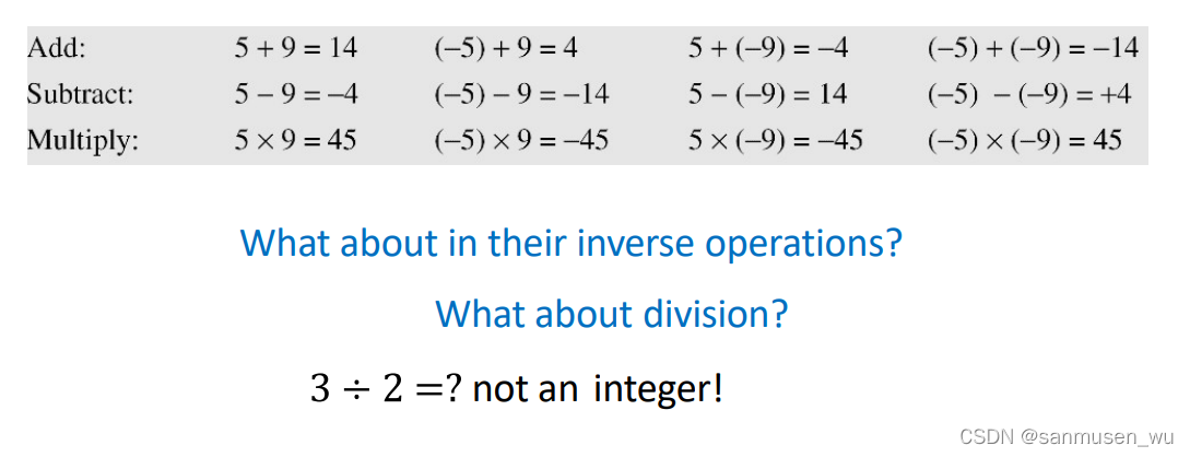
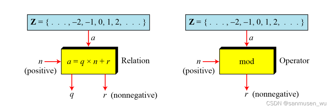
1.3. Integer Division

除法表现为乘法形式
a = q x n + r
divide a by n, we can get q and r

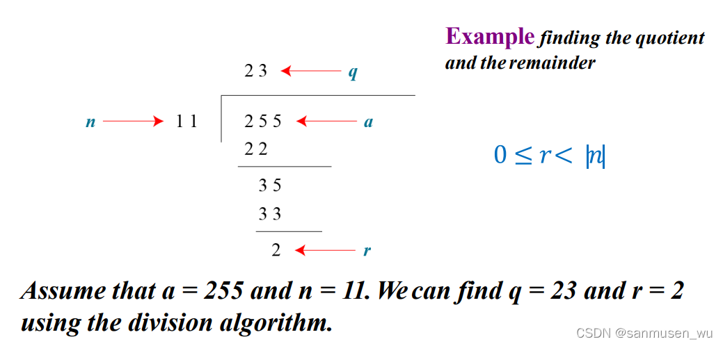
给定a和n，输出q和r

当a为负数时，r可能为负数，通过q=q-1,r=r+n来让r保持非负

r负数	r非负
-255 = (-23 x 11) + (-2)	-255 = (-24 x 11) + 9

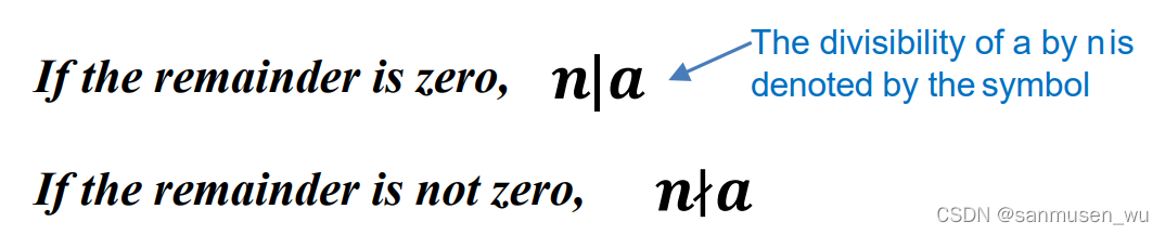
1.4. Divisibility

如果上式中a非零，r为0
a = q x n
既a可以整除(divisibility)n，写为n|a，如4|32，11|(-33)

Properties:

Property 1: if a|1, then a = ±1.
Property 2: if b|a and a|b, then a = ±b.
Property 3: if b|a and c|b, then c|a.
Property 4: if a|b and a|c, then a| (m × b + n × c), where m and n are arbitraryintegers

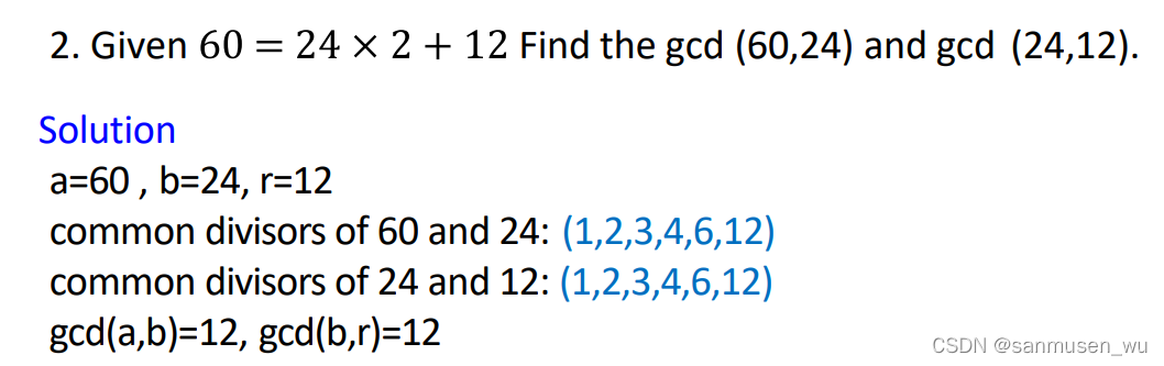
Greatest Common Divisor：最大公因数

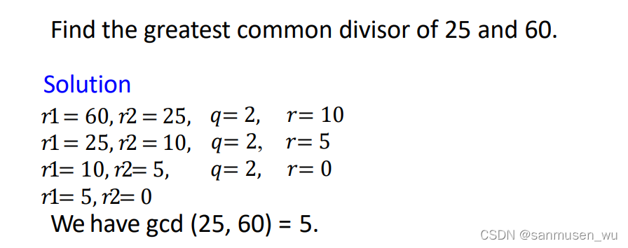
1.4.1. Euclidean Algorithm欧几里得算法/辗转相除法

形如右式：gcd(a,b)

Lemma: Let a, b, q, and r be integer such that a = bq + r and b!=0. Then gcd(a, b) = gcd(b, r).

gcd(a,0)=a, a与0的最大公因数为a

校验正确性：

Basic Euclidean algorithms：

def gcd(a,b):
	assert a>=b and b>=0 and a+b>0
	return gcd(b, a%b) if b>0 else a

用来求最大公约数的算法，迭代进行除余并辗转更新a,b和b,r。当某一轮次的b为0时a就是原先二者的最大公因数。

Note：When gcd (a, b) = 1, we say that a and b are relatively prime. 最大公因数为1，则称二者互质

算法例子：
其中r2作为下一行的r1，算出来的r作为下一行的r2.

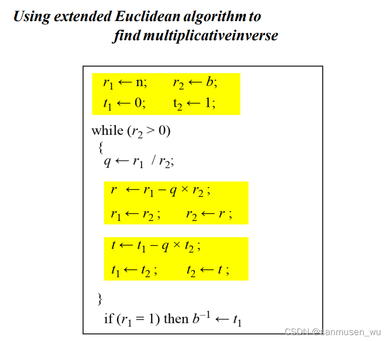
Extended Euclidean Algorithm扩展欧几里得算法：
ab的最大公因数=gcd(a,b)=s x a + t x b，其中s和t是两个整数
扩展欧几里得算法可以在算最大公因数的同时算出s和t，也可以用来计算模反元素(也叫模逆元)（下文）

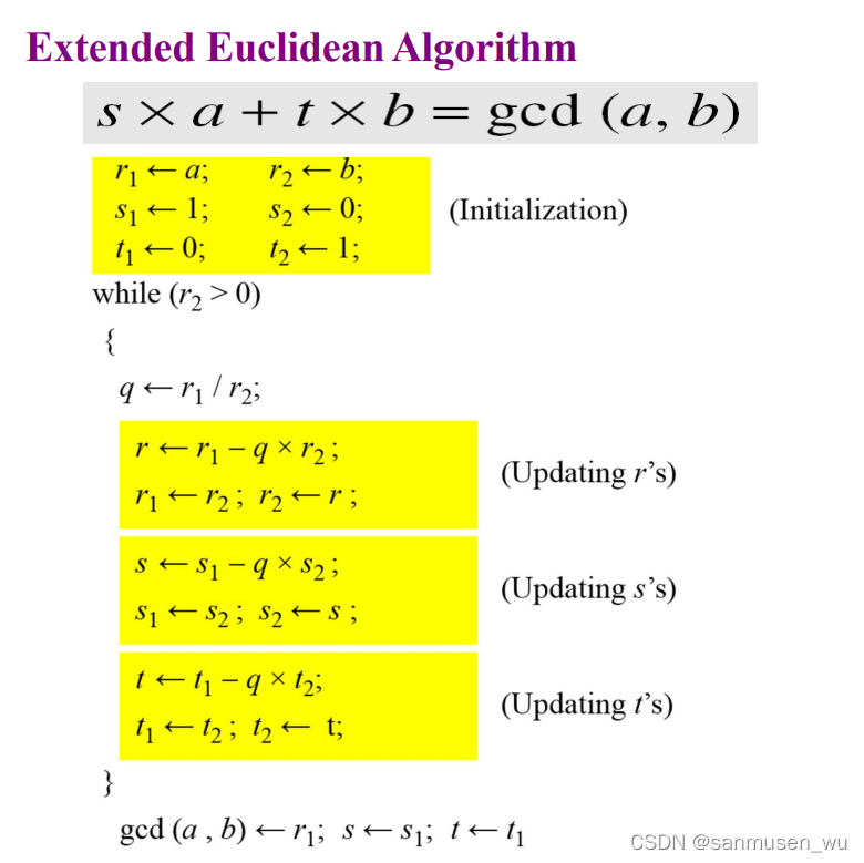
Example：
Given a = 161 and b = 28, find gcd (a, b) and the values of s and t.
Solution：
We get gcd (161, 28) = 7, s = −1 and t = 6.

2. Modular arithmetic 模运算

在模运算中，只关注remainder r。

2.1. Modulo Operator

模运算写作mod（或%），n称作modulus模数，输出r称为residue余数。

左：Division 右：Modulo

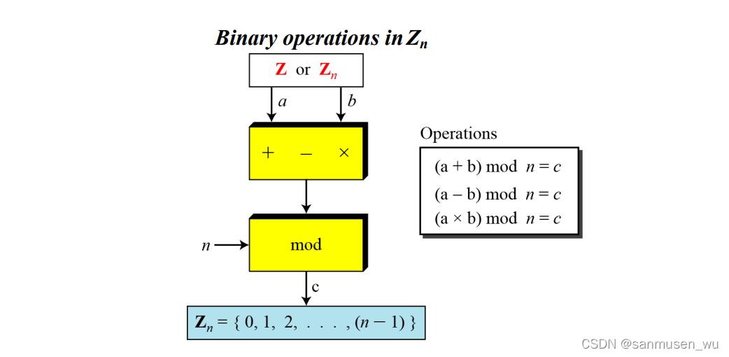
2.2. Set of Redisues

Z_n集合内包含least residues modulo n（模n后可能的最小余数们）

Z_n={ 0，1，2，3…, (n-1) }

2.3. Congruence

如果a mod m=b mod m，则称a is congruent to b modulo m，写作 a≡b(mod m)

比如：2≡12(mod 10), 8≡13(mod 5)

Residue Classes:
A residue class [a] or [a]_n is the set of integers congruent modulo n:
{… , a − 3n, a − 2n, a − n, a, a + n, a + 2n, a + 3n, …}

该类里的任意两个数都是对于模n来说congruent的。

比如：[1]₅={…, -14, -9, -4, 1, 6, 11, 16, …}

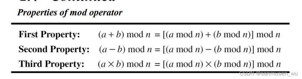
2.4. Operation in Zn

依旧是加减乘，除法在Zn集合里以模的形式表现

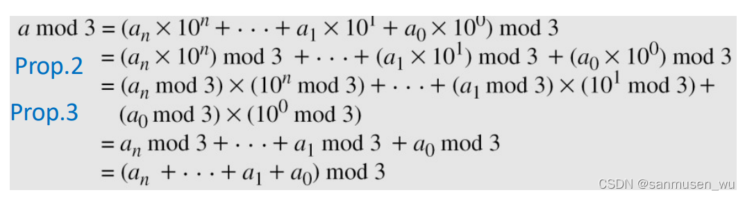
一些变换：

以及将第三条重复n次后得出： 10ⁿ mod x=(10 mod x)ⁿ

例题1：
10 mod 7=3 --> 10ⁿ mod 7 = (10 mod 7)ⁿ = 3ⁿ mod 7.

例题2：
证明一个数是否被三整除只需将各个位相加mod3

2.5. Inverse模逆元

**Additive inverse：**加法逆元
given two numbers a and b, they are additive inverse if a+b≡0(mod n)，既a+b的和模n为0。
显然在整数集合Z内对于整数n，每个数都有additive inverse。

如n=5，2的additive inverse为3，1的additive inverse 为4。

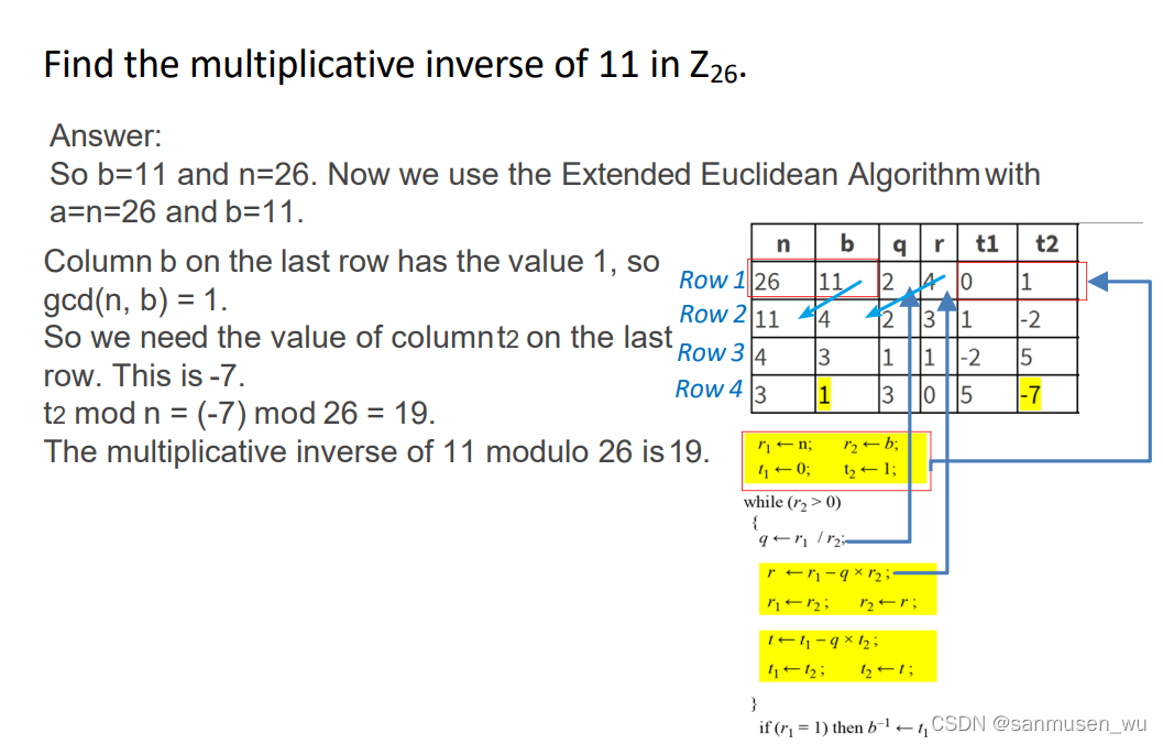
Multiplicative Inverse：乘法逆元
given two numbers a and b, they are multiplicative inverse if a * b≡1(mod n)，既ab的积mod n为1。

The extended Euclidean algorithm finds the multiplicative inverses of b in Zn when n and b are given and gcd (n, b) = 1.
The multiplicative inverse of b is the value of t after being mapped to Zn.
给定n和b，并且gcd(n, b)=1，既n和b互质，扩展欧几里得算法结束时的t映射到Z_n内得到b的模逆元

写作b^-1(mod n)

ref

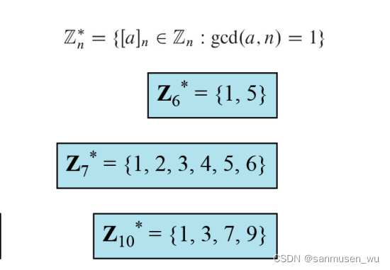
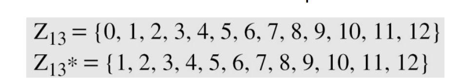
2.6. Zn*

集合Zn*表示在Zn之内与n互质的数的集合。

当n为质数时，进而有Zp和Zp*集合

3. LINEAR CONGRUENCE

Single-Variable Linear Equation：
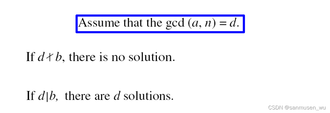
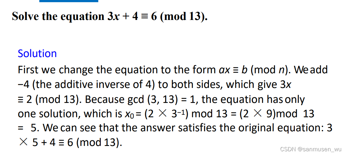
Equations of the form ax ≡ b (mod n) might have no solution or a limited number of solutions.

Example 1：
Solve the equation 10 x ≡ 2(mod 15).
Solution
First we find the gcd (10, 15) = 5. Since 5 does not divide 2, we have no solution.
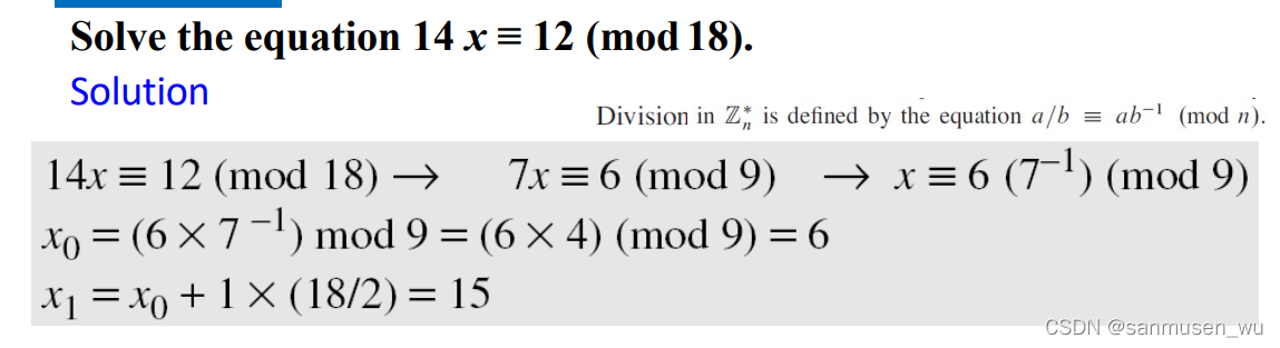
Example 3：
x0是第一个解，x1是第二个解，都在[6]₉内

Example 3：

week11

4. Modular Exponentiation

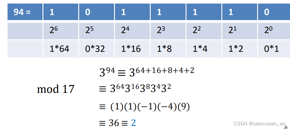
任何数字都可以表示为如下形式：
k_n2ⁿ+k_n-12^n-1+…k₁2¹+k₀2⁰
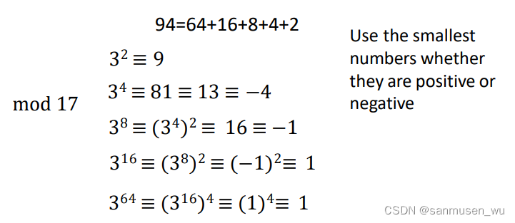
如94=64+16+8+4+2

计算3⁹⁴mod17：
3⁹⁴mod 17
=3^64+16+8+4+2mod 17
=3⁶⁴3¹⁶3⁸3⁴3² mod 17
≡ (1) (1) (−1)(−4)(9) mod 17
=36 mod 17
=2

其中：
对于3⁴ mod 17，取绝对值最小的余数-4而不是13

4.1. Euler’s function欧拉公式

Zn*（上周提到过的Zn里那些与n互质的元素）的大小表示为totient function of n: φ(n), 如果n为质数，则 φ(n)=n-1
例子：
Z₁₁* ={1,2,3,4,5,6,7,8,9,10} φ(11)=10

如果n不是质数，计算 φ(n)：
n=p₁^e1 x … x p_n ^en ，其中p为质数，e为整数
φ(n)=n*(1-1/p₁)x … x(1-1/p_n)
例子：
10=2 x 5
φ(10)=10 * (1-1/2) * (1-1/5)=4
( Z₁₀* ={1,3,7,9} φ(10)=4）

4.2. Euler’s Theorem欧拉定理

Let n be a positive integer, and let x be an integer such that gcd(x,n) = 1. Then x^φ(n)≡1 mod n.
既对于正整数n，和与其互质的整数x。那么x^φ(n) mod n =1
例子：
n=10，x=3，3^φ(10) mod 10 = 3⁴ mod 10 = 81 mod 10 = 1
n=10，x=7，7^φ(10) mod 10 = 7⁴ mod 10 = 2401 mod 10 = 1

4.3. Fermat’s Little Theorem费马小定理

Let p be prime, and let x be an intger such that x mod p ≠ 0, Then x^p-1≡1 mod p.

即：假如x是整数，p是质数，且x,p互质(即两者只有一个公约数1)，那么x^(p-1) mod p=1。
例：p=5，1⁴ mod 5 = 1, 3⁴ mod 5 = 1

Corollary:

Let p be prime. For each nonzero residue x in Z_p, the multiplicative inverse of x is x^p-2 mod p
既：假如x是不大于p的正整数，p是质数。x^-1 ≡x^p-2 (mod p)
Proof:
x(x^p-2 mod p) mod p=x^p-1 mod p = x^p-1 mod p = 1

4.4. if n is prime?

Let n > 0 be an integer. How to find out if n is prime? This is a central questionin cryptographic computations.

4.5. Encryption schemes/ciphers

把原文M称为plaintext，加密后的密文C称为ciphertext

4.5.1. symmetric encryption对称加密

发送者发送前把原文加密，通过不安全信道传输给接收者，接收者再把密文解密成原文。

secret key密钥K被两者所使用。

Substitution ciphers替换加密法：

1. 此时加密密钥是字母间映射的permutation偏移。如A换成D，B换成H。
   解密既反向映射字母。如D换成A，H换成B
2. The Caesar cipher 凯撒加密既是替换加密，密钥K代表偏移量，P明文，C密文，字母用视作数字。加密：C[i]=P[i]+K mod m, 解密：P[i] = C[i]-K mod m
3. 替换加密非常不安全，通过频率分析出现的多的词能够知道K
   

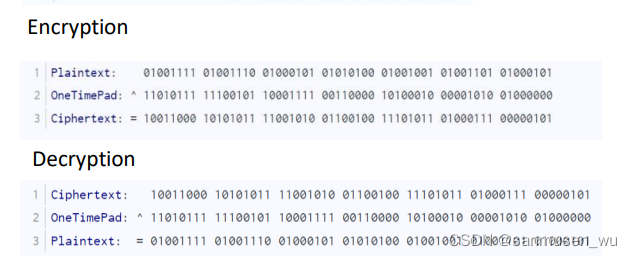
The One-time pad一次性密钥：

1. 双方使用一个共同的随机生成的, 长度等于信息长度的, 一次性的比特密钥K，
2. 加密encrypt：密文等于原文按位异或/exclusive or/Xor密钥，C=M⊕K。（1⊕1=0⊕0=0,1⊕0=1，或者bit_p+bit_k mod 2=bit_c)
3. 解密decryption: 密文再次按位异或密钥即可还原：
   bit_c⊕bit_k = bit_p⊕(bit_k⊕bit_k) = bit_p⊕0 = bit_p
4. 例子：
   
5. 优点：安全（密钥完全随机的情况下），快（异或）
6. 缺点：密钥K必须和原文一样大，密钥只能用一次。

ref

4.5.2. 非对称加密

非对称加密体系通过公钥私钥的方式解决了对称加密的密钥分发问题（既发送接收者双方都要有同一个密钥）。

A public-key cryptosystem consists of an encryption function E（公钥） and a decryption function D（私钥）. For any message M, the following properties musthold:

1. D(E(M)) = M.
2. Both E and D are easy to compute.
3. It is computationally infeasible to derive D from E.
4. E(D(M)) = M.

第三点从加密方法无从得知解密方法，意味着只有拥有解密方法的人才能解密密文，因此E也被称为单向函数。

RSA
选择两个大质数p，q：n=p*q, 定义φ(n)=(p-1)(q-1)
选择两个数字e和d：使得 gcd(e,φ(n))=1 和 ed mod φ(n) = 1 （既d是e的乘法逆）

加密：C←M^e mod n, 公钥包含e,n，公钥是公开的，想要发送给A的信息都可以使用A的公钥加密。
解密：M←C^d mod n, 私钥包含d,n，私钥只有A自己拥有，使用A的公钥加密的信息只有A使用自己的私钥才能解密。

合理性：对于任意0<x<n和符合的e,d，x^ed≡ x (mod n)

例子：p=7, q=17, n=119, φ(n)=96, e=5, d=77
加密M=19，C=19⁵ mod 119 = 66
解密M=66⁷⁷ mod 119 = 19

身份验证功能：假如A要验证B的身份，A只需要发送给B一段明文M。B使用自己的密钥将M加密发送给A，A使用B的公钥可以解密这个密文来验证B确实拥有B的密钥。

公钥和私钥在于公开性的差别，事实上可以公钥加密私钥解密(加密通信），也可以私钥加密公钥解密（身份验证）。

RSA使用上的困难：
计算量大：要计算x^e mod n的结果

1. 平方，如计算x¹⁶，可以先计算x²,再算 (x²)²…
2. 另一种方法使用上文提到的Modular Exponentiation，既将数字e拆成2的多项式相加的形式
   

破解RSA的困难性：
已知公钥e和n，要想求出私钥d，由于ed=φ(n)k+1，k是个未知整数。要得到φ(n)，必须知道p,q。由于n=p*q，只有将n因式分解才能算出可能的p，q。

ref

week12

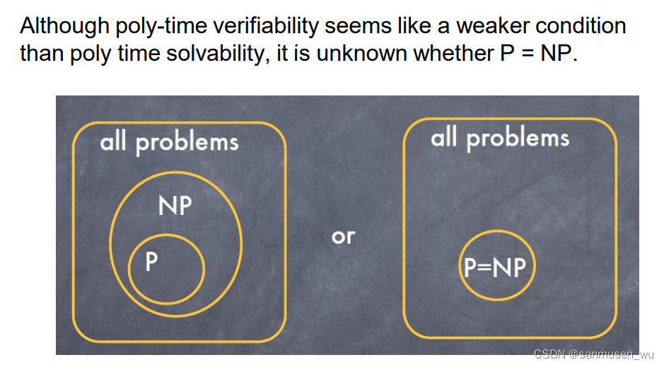
NP=P? or NP!=P

引子：假如现在要给几百人分配进若干间三人房，同时给定一个禁止名单指示若干人员组合，要求那些人员不能被分配到同一个房间，如果禁止名单里的人分到同一房间，则称这种分配failed。
分析：如果给定一种房间分配名单，我们能够很快地检查出这个名单是否failed。
但是除了遍历所有结果，我们很难找到一种方便的方法从0开始找到一种有效的房间分配名单。
问题：是方便的方法 很难找到 还是 这种方法不存在

{0, 1} Knapsack 01背包问题

Input: A collection of items { i1,i2,… in} where item i_j has integer weight w_j > 0 and gives integer benefit b_j . Also, a maximum weight W.
Goal: Find a subset of the items whose total weight does not exceed W and that maximizes the total benefit (taking fractional parts of items is not allowed).
Note: The dynamic programming algorithm for the { 0,1} Knapsack problem runs in time O((nW), which is not polynomial in the size of the problem.

polynomial time多项式时间 VS pseudo-polynomial伪多项式时间：
求算法时间复杂度和其输入的关系，输入可以分为：输入的逻辑大小（列表长度） 和 输入的物理大小（占多少比特来存储）
背包问题的dp解时间复杂度是O(nW)，是多项式级，这里输入是逻辑大小
对于一个大小为W的数，需要长度i=log₂W的比特位来存储，W=2ⁱ
则对于物理输入大小来说，时间复杂度是O(n * 2ⁱ)，是指数级。
对于这种逻辑输入大小而言是多项式级，物理输入大小而言非多项式级的称为 伪多项式时间

Decision/Optimization problems

Decision 决策问题： 给定一输入，判断是否
Optimization 优化问题： 得到最大化/最小化某值
优化问题可以转化为决策问题：给定一输入k，判断是否有解大于/小于k
如果能高效地回答决策问题，则我们能高效地解决优化问题

Example:
Optimization problem: Let G be a connected graph with integer weights on its edges. Find the weight of a minimum spanning tree in G.
Decision problem: Let G be a connected graph with integer weights on its edges, and let k be an integer. Does G have a spanning tree of weight at most k?

P and NP

什么是P,NP,NPC,NP-hard问题

假设某问题X的输入被编码为二进制字符串s，长度为|s|，算法A能接受某些s并返回true。L(X)为这个问题中所有被A接受的s的集合，L(X)也被称为language语言。

P

The complexity class P is the set of all decision problems X that can be solved in worst-case polynomial time.P集合表示所有能在多项式时间内解决的问题

That is, there is an algorithm A that if s ∈ L(X), then on input s, A outputs “yes” in time p(|s|), where |s| is the length of s, and p(·) is a polynomial.

• fractional knapsack
• shortest paths in graphs with non-negative edgeweights,
• task scheduling.

Efficient certification

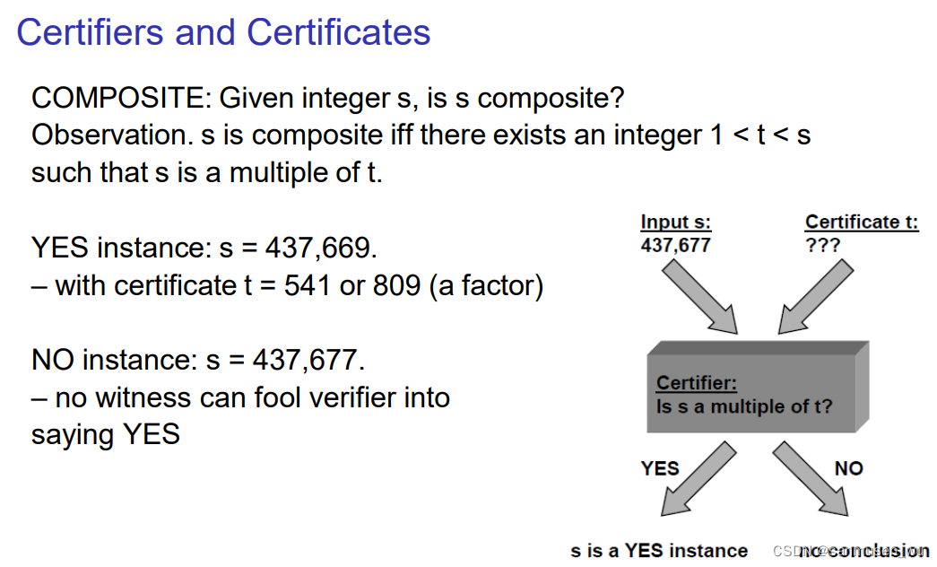
Example: { 0,1} Knapsack Problem
Given a collection of weights, benefits, and parameters W and k for an instance of the { 0,1} Knapsack Problem, if I propose a subset of these items, it is easy to check if those items have total weight at most W and if the total benefit is at least k.
如果给定若干个背包问题的解，很容易检查这些解的重量是否不超过W并且价值最少是k

If both of those conditions are satisfied, then we say that the subset of items is a certificate for the decision problem, i.e. it verifies that the answer to the { 0,1} Knapsack decision problem is “yes.”

The idea of efficient certification is what is used to define the class of problems called NP.

input：问题的输入
certificate：可以辅助证明输入是否通过决策器的变量
verify：certificate能够证实这个input的输出为Y/N
certifier：决策器

deterministically确定性算法 VS non-deterministically非确定性算法

确定性算法：给定一个输入，只有一种最终结果，如计算数组总和
非确定性算法：给定一个输入，过程中会有多种分支，如求解数独

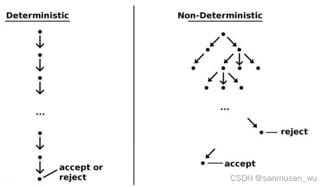
NP (non-deterministic polynomial time)

P类问题、NP类问题和NPC类问题

• The class NP consists of all decision problems for which there exists an efficient certifier.（高效指 指数级时间）

There is a polynomial function q(·) so that for every string s, we have s ∈ L(X) if and only if there exists a string t such that |t| ≤ q(|s|) and B(s,t) = “yes”.

另一种定义：

• The class NP is the set of decision problems X (or languages L(X )) that can be non-deterministically accepted in polynomial time.

“一个多项式不确定算法是一个两阶段的过程，它把一个判定问题的实例l作为它的输入，并进行下面的操作：
(1)非确定（“猜测”）阶段：生成一个任意串S，把它当作给定实例l的一个候选解。
(2)确定(“验证”)阶段：确定算法把l和S都作为它的输入，如果S可被证明是l的一个解，就在多项式时间内输出“是”（如果S不是l的一个解，该算法要么返回“否”，要么根本不停下来）。”

Thus NP can also be thought of as the class of problems whose solutions can be verified in polynomial time. NP为能在多项式时间验证其解的问题

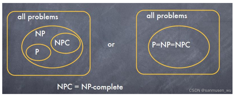
P ⊆ N P

如果能在多项式时间内给出问题的解，那么就能在多项式时间内判别问题。

Boolean Satisfiability Problem（SAT）

左侧有若干输入，中间若干逻辑门，右侧一个输出

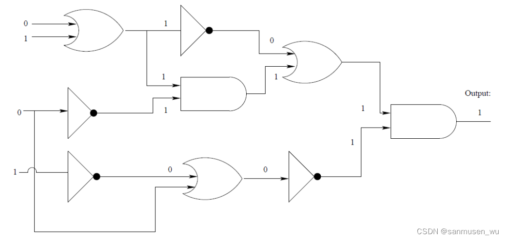
Input: a Boolean Circuit with a single output vertex
Question: is there an assignment of values to the inputs so that the output value is 1?

A non-deterministic algorithm chooses an assignment of input bits and checks deterministically whether this input generates an output of 1.非确定性算法选择输入位的分配，并确定性地检查此输入是否生成1的输出

SAT: Satisfiability可满足性
术语“可满足”的含义是存在一组“真值赋值truth assignment”使布尔表达式为真。

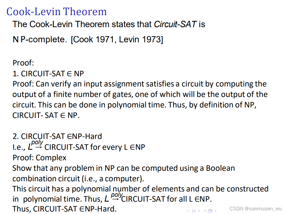
Proof: We construct a nondeterministic algorithm for accepting CIRCUIT-SAT in polynomial time. 
We first use the choose method to "guess "the values of the input nodes as well as the output value of each logic gate. 
Then, we simply visit each logic gate g in C, that is, each vertex with at least one incoming edge. 
We then check that the guessed value for the output of g is in fact the correct value for g's Boolean function, be it an AND, OR, or NOT, based on the given values for the inputs for g. 
This evaluation process can easily be performed in polynomial time. If any check for a gate falls, or if the guessed value for the output is 0, then we output "no". 
If, on the other hand, the check for every gate succeeds and the output11, the algonthm outputs yes. 
Thus, if there is indeed a satisfying assignment of input values for C then there is a possible collection of outcomes to the choose statements so that the algorithm will output "yes"in polynomial time. 
Likewise, if there is a collection of outcomes to the choose statements so that thle algonthm outputs yes in polynomial time algorithm, 
there must be a satisfying assignment of input values for C. Therefore. CIRCUIT-SAT is in NP

Vertex Cover (VC)

顶点覆盖问题

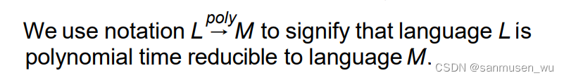
Polynomial-time reducibility多项式规约

We say that a language L, defining some decision problem, is polynomial-time reducible to a language M, if:
there is a function f , computable in polynomial time,that takes as an input s ∈ L, and transforms it into a input f (s) ∈ M such that s ∈ L if and only if f (s) ∈M.
我们可以将一个决策问题的输入转换为另一个决策问题的适当输入。此外，当且仅当第二个决策问题有一个“是”的解决方案时，第一个问题才有一个“是”的解决方案。

“例如求解一元一次方程这个问题可以约化为求解一元二次方程，即可以令对应项系数不变，二次项的系数为0，将A的问题的输入参数带入到B问题的求解程序去求解。”

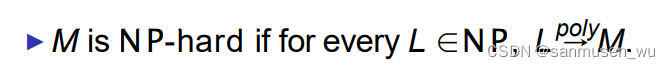
NP-hard

We say that a language M, defining some decision problem, is NP-hard if every other language L in NP is polynomial-time reducible to M. So this means that
NP-hard指可以被NP问题多项式归约到的问题。
优化求解中的NP-hard 问题学习

NP-complete

If a language G is NP-hard and it belongs to NP itself, then G is NP-complete.
NP-complete指在NP-hard中并在NP中的问题。
NP-complete problems are some of the hardest problems in NP.

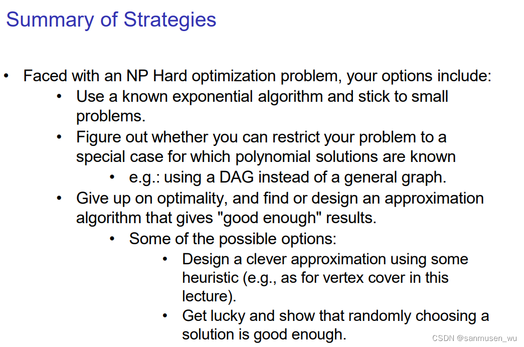
Pragmatic approach务实的方法:
If your problem is NP-complete, then don’t waste time looking for an efficient algorithm, focus on approximations or heuristics.
如果一个问题是NPC问题，那么试图使用近似解法或启发式解法

如何证明一个问题X是NP完全的（NP-complete）：

1. show that X ∈ NP, i.e. show that X has a polynomial-time nondeterministic algorithm, or equivalently, show that X has an efficient certifier。先证明能多项式时间内判别问题的解
2. take a known NP-complete problem Y , and demonstrate a polynomial time reduction from Y to X , i.e. show that Y → X. 找到一个NPC的问题Y，使得Y能多项式规约到X

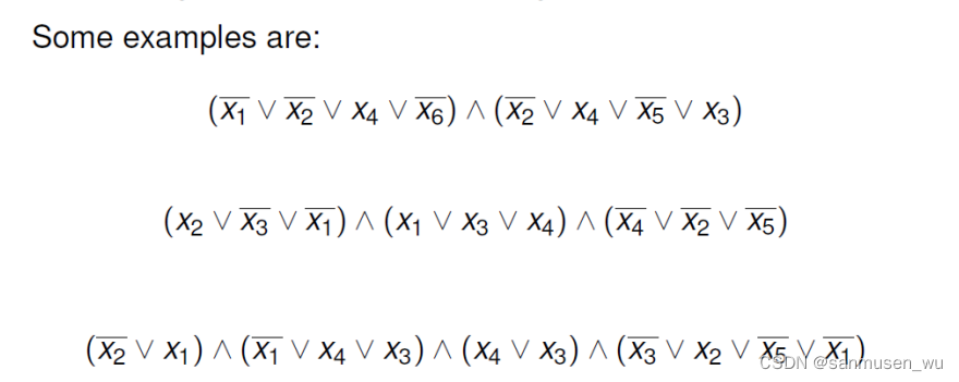
Conjunctive Normal Form合取范式CNF

与∧ 或∨ 非－

CNF-SAT

Input: A Boolean formula in CNF.
Question: Is there an assignment of Boolean values to its variables so that the formula evaluates to 1 (i.e. is the formula satisfiable)? 是否有x集合使总结果为1

3-SAT

Input: A CNF C = c₁ ∧ c₂ ∧ . . . ∧ c_m of clauses dependent on variables x₁, x₂,…,x_m such that each c_i is of the form x_i1 ∨ x_i2 ∨ x_i3 for 1 ≤ i ≤m.
Question: Is there a truth assignment for variables xi that satisfies C?

合取范式就是⼀种所有⼦句都由合取（即“与”）联接所构成的公式，如"a & (!b | c) & (a | !c | d)"， 组成⼦句的a, !b, c, !c, d就是“⽂字”。3合取范式”就是每个子句恰好由3个⽂字所组成的合取范式。

*举个例子：小红，小王，小江等n⼈想找个地⽅去做运动，他们觉得这个地方可能会有m种情况。为了尽量满足所有人的癖好，每个人都根据可能出现的情况提了⼀个包含3个需求的列表：小红想找个“有窗户”或者“有厕所”或者“没臭味”的地小，小王想找个“没窗户”或“有臭味”或“没厕所”的地小，小江想找个“有厕所”或“没臭味”或“没窗户”的地⽅
问，是否存在⼀个地方可以满足所有⼈的（⾄少⼀个）要求？

如果最后找到了⼀个“有窗户，没厕所，没臭味”的地⽅，那么“有窗户，没厕所，没臭味”就是变量的真值赋值。
所有⼈需求就是合取范式，如果“每个人的需求都有3项且⾄少要满足1项”就是“3合取范式”。*
链接

3-SAT is CNF-SAT in which each clause has exactly three literals.

Theorem: 3-SAT is N P-complete.

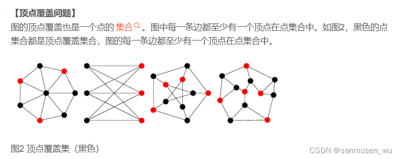
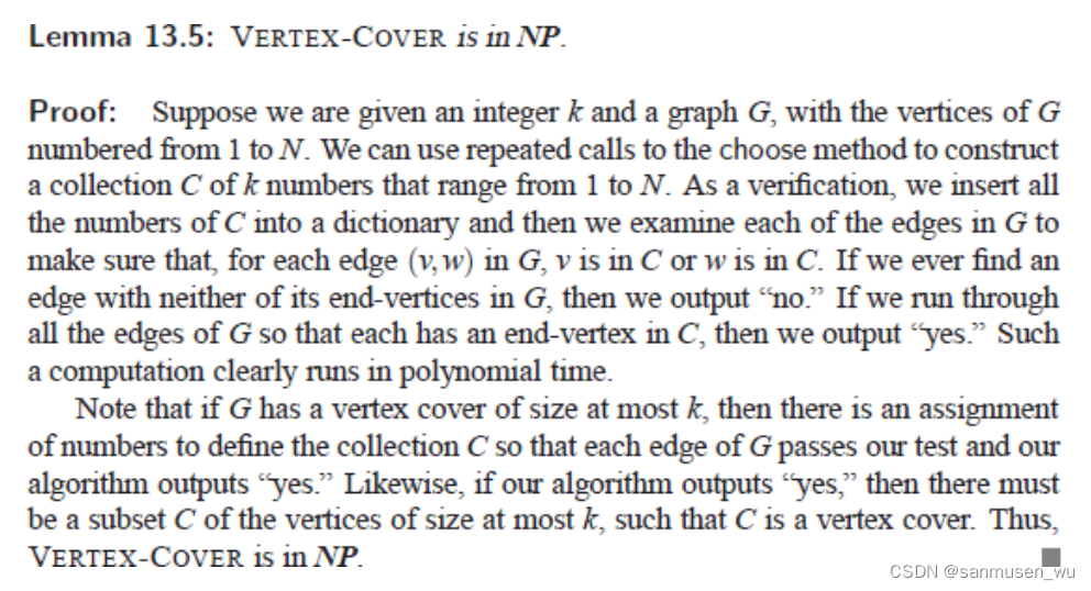
Vertex Cover (VC)

是否有大小为k的点集使得顶点全覆盖
Theorem: VC is N P-complete.

3-Coloring of Graphs

Input: A graph G.
Question: 每个点分配1，2，3三种标签，是否有种分配方式使得相邻点的标签不同。
If k ≥ 3, then k -COL is NP-complete.

week13

Optimization Problems

对于一个问题实例x，有许多可行解s组成的集合F(x)，试图找到一个解使某一个代价函数c()最大/小, OPT(x)=min or max {c(s)：s∈F(x)} , 最优化问题基本上是NPC问题。

• 最小生成树
• 最小顶点覆盖

Approximation Ratios

衡量近似解T(x)与最优解OPT(x):

最小化问题 c(T(x))/c(OPT(x))=r
最大化问题 c(OPT(x))/c(T(x))=r

T is a k-approximation to the optimal solution OPT if r<=k
如果r<=k，则称T k近似于 最优解OPT，其中k不小于1，r越小越好，r=1的话就是最优解法了

Polynomial-Time Approximation Schemes

A problem L has a polynomial-time approximation scheme (PTAS) if it has a polynomial time (1+Є)-approximation algorithm, for any fixed Є>0 (this value can appear in the running time).

Fully Polynomial-Time Approximation Schemes

We have fully polynomial-time approximation scheme when its running time is polynomial not only in n but also in 1/Є，指时间复杂度与1/Є有关。

For example its running time could be O((1/Є)³n²).

Vertex Cover顶点覆盖近似解

G = (V, E): a subset V′ ⊆ V such that if (u, v) ∈ E then u ∈ V′ or v ∈ V′ or both (there is a vertex in V′ “covering” every edge in E).
• OPT-VERTEX-COVER: Given an graph G, find a vertex cover of G with smallest size.
• OPT-VERTEX-COVER is NP-hard.

• Approx-Vertex-Cover近似顶点覆盖：
维护边集，每次选择一条边，将其两顶点加入目标点集C，在边集中去除所有与这两点相邻的边

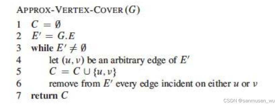
这个解法是2-approximation的，证明如下
Let A be the set of edges chosen in line 4 of the algorithm. Any vertex cover must cover at least one endpoint of every edge in A.
• No two edges in A share a vertex, because for any two edges one of them must be selected first (line 4), and all edges sharing vertices with the selected edge are deleted from E′ in line 6, so are no longer candidates on the next iteration of line 4.
• Therefore, in order to cover A, the optimal solution C* must have at least as many vertices as edges in A:
| A | ≤ | C* |
Since each execution of line 4 picks an edge for which neither endpoint is yet in C and line 5 adds these two vertices to C, then we know that: | C | = 2 | A |
• Therefore: | C | ≤ 2 | C* |
• That is, |C| cannot be larger than twice the optimal, so is a 2- approximation algorithm for Vertex Cover.
• This is a common strategy in approximation proofs: we don’t know the size of the optimal solution, but we can set a lower bound on the optimal solution and relate the obtained solution to this lower bound.

P	NP	NP-hard	NP-complete
能在多项式时间内解决	能在多项式时间内判定一个解是否正确。用非确定算法在非多项式时间内选定解，确定算法在多项式时间内判断解的正确与否	NP问题规约到NP-hard，但不一定在多项式内可判定	既是NP-hard又是NP问题，在多项式时间内可判定
排序算法，部分背包问题	旅行商问题，01背包问题，SAT可满足性问题，3-SAT，VC顶点覆盖问题，三色图问题	SAT可满足性问题，3-SAT，VC顶点覆盖问题，三色图问题	SAT可满足性问题，3-SAT，VC顶点覆盖问题，三色图问题
证明多项式时间可解决	证明多项式时间内可判定一个解	证明由某NP问题规约来	证明多项式时间内可判定，然后找到一个NPC问题，并且证明那个NPC问题可以规约到这个问题上