control theory-优化控制算法

0.建模

控制前,需要对系统建模

我们以最简单的倒立摆为例：

a.特点+目标+原理

特点：非线性、高阶次、多变量；
目标：通过给小车底座加力 F（控制量），使小车停留在预定的位置，并使摆杆不倒下，即不超过预先定义的竖直偏离角度范围。
原理：小车位置编码器将小车的位移和速度信号反馈给运动控制卡，角度编码器将摆角的角度、角速度信号反馈给运动控制卡。计算机从运动控制卡中读取实时反馈数据，确定小车向哪个方向移动、移动速度、加速度等，产生相应的控制量 F

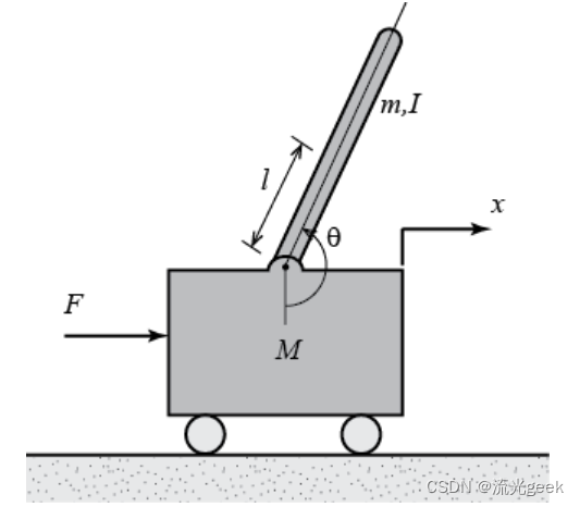
b.系统变量+系统受力分析

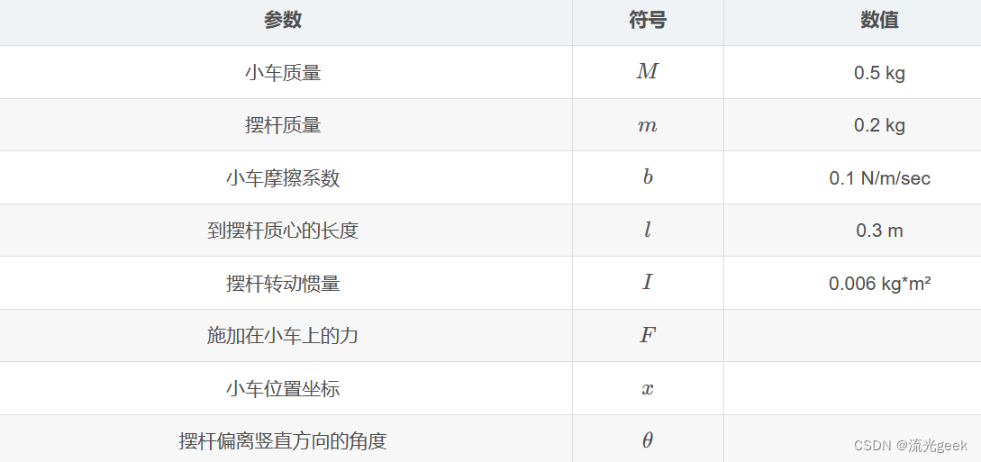
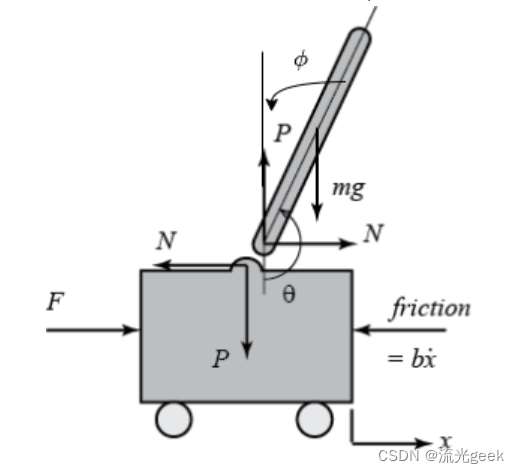
根据所取变量，一种取钝角θ为变量建立系统方程组，另一种以锐角ϕ为变量建立系统方程组

我们以锐角ϕ为变量建立系统模型，这里的ϕ为 π − θ，刚体绕定轴转动动力学方程需要规定正方向，一般取逆时针方向为正方向：

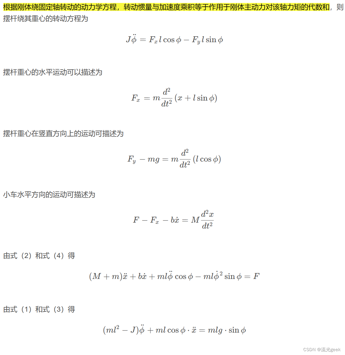
系统模型建立完毕（注意，可以选取钝角θ来建立，或者取顺时针为正方向建立）

c.动力学方程雅可比线性化

雅可比矩阵是一种线性化工具，用来近似描述非线性系统在其邻域内的行为。在机器人学和控制理论中，这种方法特别有用，它允许我们通过线性化来简化对系统的分析，如稳定性、能控性的分析

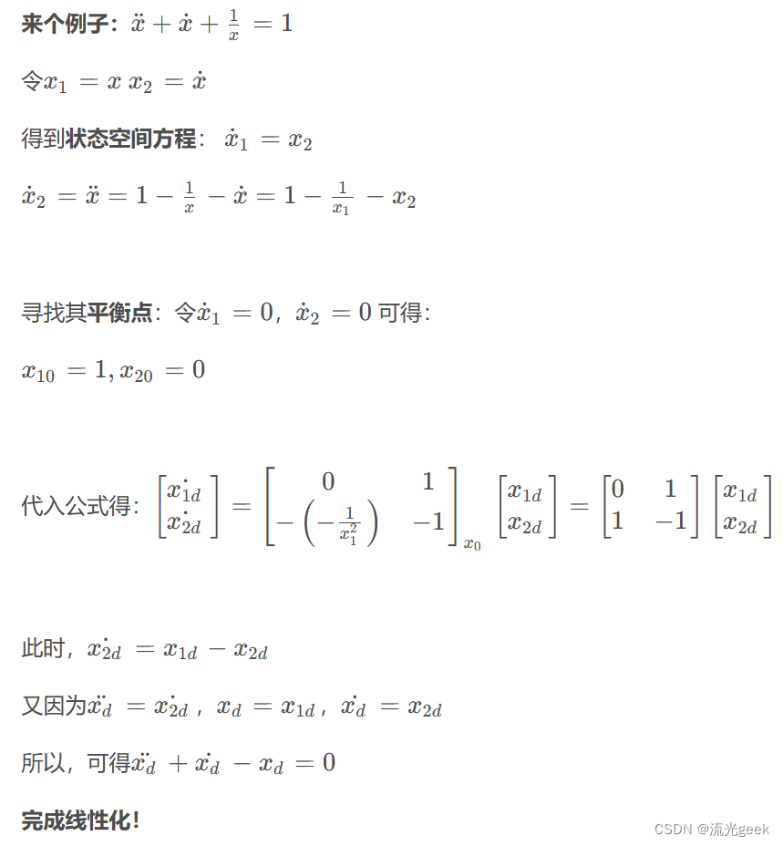
对于倒立摆：

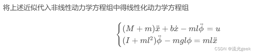
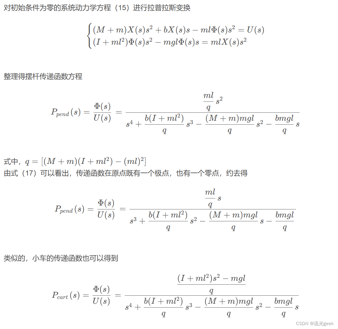
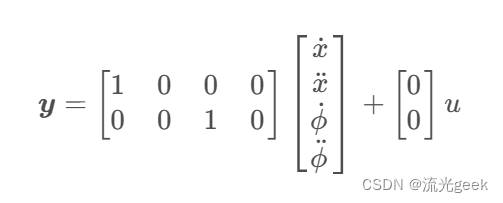
d.传递函数&状态空间

传递函数：传递函数是经典控制理论的工具，只能用于SISO和LTI系统，它是控制系统在复数域的数学模型

状态空间：状态空间模型属于现代控制理论，对SISO和MIMO、LTI和非线性或时变系统都适用，它是描述动态系统的另一种数学模型

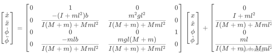
matlab for 状态空间方程：

M = .5;
m = 0.2;
b = 0.1;
I = 0.006;
g = 9.8;
l = 0.3;

p = I*(M+m)+M*m*l^2; %denominator for the A and B matrices

A = [0      1              0           0;
     0 -(I+m*l^2)*b/p  (m^2*g*l^2)/p   0;
     0      0              0           1;
     0 -(m*l*b)/p       m*g*l*(M+m)/p  0];
B = [     0;
     (I+m*l^2)/p;
          0;
        m*l/p];
C = [1 0 0 0;
     0 0 1 0];
D = [0;
     0];

states = {'x' 'x_dot' 'phi' 'phi_dot'};
inputs = {'u'};
outputs = {'x'; 'phi'};

sys_ss = ss(A,B,C,D,'statename',states,'inputname',inputs,'outputname',outputs)

1.LQR for 倒立摆（python）

LQR:

state-x,action-u

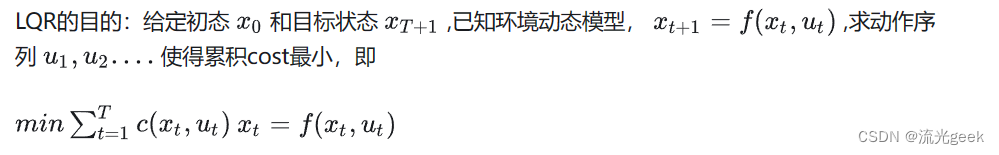
(目标状态已知)

控制theory:R和Q矩阵分别表示在最优化的代价函数中控制输入和误差的相对权重，Q,R矩阵也是cost function的一部分；A,B,C,D矩阵（空间状态方程模型）：A 是系统的状态矩阵，B 是系统的控制输入矩阵，C 是系统的输出矩阵，D 是系统的直接传递矩阵

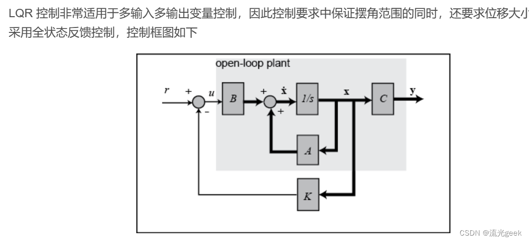
直接目标：需要确定状态反馈矩阵（向量）K

系统变量：M=1  m=0.3(g取9.8)  L=2

def main():模拟展示倒立摆的控制和运动过程，x0 是系统初始状态的数组，包含了小车的位置（x坐标）和倒立摆的角度（theta)等等

杆的位移𝑥1 - 初始值为 0.0

杆的速度𝑥2- 初始值为 0.0

杆的角度𝑥3 - 初始值为 0.3，这意味着杆在初始时稍微偏离直立状态。

杆的角速度𝑥4 - 初始值为 0.0

time设置为0，表示模拟时间的起点。sim_time是预定的总模拟时间,delta_t 是每次模拟时间步长

当模拟时间time小于sim_time时，持续执行循环，time += delta_t;每次迭代，时间time增加一个delta_t，u = lqr_control(x)计算控制输入u，通常使用线性二次调节（LQR）控制算法，根据当前系统状态x来确定。x = simulation(x, u)：根据当前状态x和控制输入u，执行一次模拟步骤，更新系统状态x

                    
def get_model_matrix():计算出A,B矩阵，为倒立摆系统提供一个状态空间模型，状态矩阵A 定义了系统状态随时间的变化。对于一个简单的倒立摆，控制输入矩阵 B 定义了控制输入 u（在这个例子中是控制力矩）如何影响系统的状态（无C,D，在这个例子中，我们不关注输出）

def simulation(x, u):计算下一个状态x

def solve_DARE(A, B, Q, R, maxiter=150, eps=0.01):迭代法计算Pn直到收敛,解出P

def dlqr(A, B, Q, R):解出P和增益矩阵K以及特征值

def lqr_control(x):计算LQR控制器的控制输入 u (u=−K⋅x)，用于倒立摆系统(dlqr函数，准确地说是solve_DARE函数首先求解出离散时间代数Riccati方程以获取状态反馈增益矩阵 K）

import math
import time

import matplotlib.pyplot as plt
import numpy as np
from numpy.linalg import inv, eig

# Model parameters

l_bar = 2.0  # length of bar
M = 1.0  # [kg]
m = 0.3  # [kg]
g = 9.8  # [m/s^2]

nx = 4  # number of state
nu = 1  # number of input
Q = np.diag([0.0, 1.0, 1.0, 0.0])  # state cost matrix
R = np.diag([0.01])  # input cost matrix

delta_t = 0.1  # time tick [s]
sim_time = 5.0  # simulation time [s]

show_animation = True


def main():
    x0 = np.array([
        [0.0],
        [0.0],
        [0.3],
        [0.0]
    ])

    x = np.copy(x0)
    time = 0.0

    while sim_time > time:
        time += delta_t

        # calc control input
        u = lqr_control(x)

        # simulate inverted pendulum cart
        x = simulation(x, u)

        if show_animation:
            plt.clf()
            px = float(x[0, 0])
            theta = float(x[2, 0])
            plot_cart(px, theta)
            plt.xlim([-5.0, 2.0])
            plt.pause(0.001)

    print("Finish")
    print(f"x={float(x[0, 0]):.2f} [m] , theta={math.degrees(x[2, 0]):.2f} [deg]")
    if show_animation:
        plt.show()


def simulation(x, u):
    A, B = get_model_matrix()
    x = A @ x + B @ u

    return x


def solve_DARE(A, B, Q, R, maxiter=150, eps=0.01):
    """
    Solve a discrete time_Algebraic Riccati equation (DARE)
    """
    P = Q

    for i in range(maxiter):
        Pn = A.T @ P @ A - A.T @ P @ B @ \
            inv(R + B.T @ P @ B) @ B.T @ P @ A + Q
        if (abs(Pn - P)).max() < eps:
            break
        P = Pn

    return Pn


def dlqr(A, B, Q, R):
    """
    Solve the discrete time lqr controller.
    x[k+1] = A x[k] + B u[k]
    cost = sum x[k].T*Q*x[k] + u[k].T*R*u[k]
    # ref Bertsekas, p.151
    """

    # first, try to solve the ricatti equation
    P = solve_DARE(A, B, Q, R)

    # compute the LQR gain
    K = inv(B.T @ P @ B + R) @ (B.T @ P @ A)

    eigVals, eigVecs = eig(A - B @ K)
    return K, P, eigVals


def lqr_control(x):
    A, B = get_model_matrix()
    start = time.time()
    K, _, _ = dlqr(A, B, Q, R)
    u = -K @ x
    elapsed_time = time.time() - start
    print(f"calc time:{elapsed_time:.6f} [sec]")
    return u


def get_numpy_array_from_matrix(x):
    """
    get build-in list from matrix
    """
    return np.array(x).flatten()


def get_model_matrix():
    A = np.array([
        [0.0, 1.0, 0.0, 0.0],
        [0.0, 0.0, m * g / M, 0.0],
        [0.0, 0.0, 0.0, 1.0],
        [0.0, 0.0, g * (M + m) / (l_bar * M), 0.0]
    ])
    A = np.eye(nx) + delta_t * A

    B = np.array([
        [0.0],
        [1.0 / M],
        [0.0],
        [1.0 / (l_bar * M)]
    ])
    B = delta_t * B

    return A, B


def flatten(a):
    return np.array(a).flatten()


def plot_cart(xt, theta):
    cart_w = 1.0
    cart_h = 0.5
    radius = 0.1

    cx = np.array([-cart_w / 2.0, cart_w / 2.0, cart_w /
                   2.0, -cart_w / 2.0, -cart_w / 2.0])
    cy = np.array([0.0, 0.0, cart_h, cart_h, 0.0])
    cy += radius * 2.0

    cx = cx + xt

    bx = np.array([0.0, l_bar * math.sin(-theta)])
    bx += xt
    by = np.array([cart_h, l_bar * math.cos(-theta) + cart_h])
    by += radius * 2.0

    angles = np.arange(0.0, math.pi * 2.0, math.radians(3.0))
    ox = np.array([radius * math.cos(a) for a in angles])
    oy = np.array([radius * math.sin(a) for a in angles])

    rwx = np.copy(ox) + cart_w / 4.0 + xt
    rwy = np.copy(oy) + radius
    lwx = np.copy(ox) - cart_w / 4.0 + xt
    lwy = np.copy(oy) + radius

    wx = np.copy(ox) + bx[-1]
    wy = np.copy(oy) + by[-1]

    plt.plot(flatten(cx), flatten(cy), "-b")
    plt.plot(flatten(bx), flatten(by), "-k")
    plt.plot(flatten(rwx), flatten(rwy), "-k")
    plt.plot(flatten(lwx), flatten(lwy), "-k")
    plt.plot(flatten(wx), flatten(wy), "-k")
    plt.title(f"x: {xt:.2f} , theta: {math.degrees(theta):.2f}")

    # for stopping simulation with the esc key.
    plt.gcf().canvas.mpl_connect(
        'key_release_event',
        lambda event: [exit(0) if event.key == 'escape' else None])

    plt.axis("equal")


if __name__ == '__main__':
    main()

注：此例未设置目标状态，但在使得cost function最小的过程中，为使状态最小，最终是杆直立状态。x-状态（的）成本，u-输入（的）成本

result（最终系统稳定即达到了杆直立，杆的角度接近或等于 0°）:

2.ILQR for 倒立摆（python）

3.MPC for 四旋翼无人机（python)

4.ILQR for panda robot arm(python+pybullet+pinocchio)

5.c++从零实现mpc