机器学习：gastric.xlsx数据集文本分类

文章节选自我的课程论文：

本文研究了针对gastric.xlsx数据集的文本分类算法。该数据集包含250个胃部活检报告样本，涵盖了不同病理特征的描述。

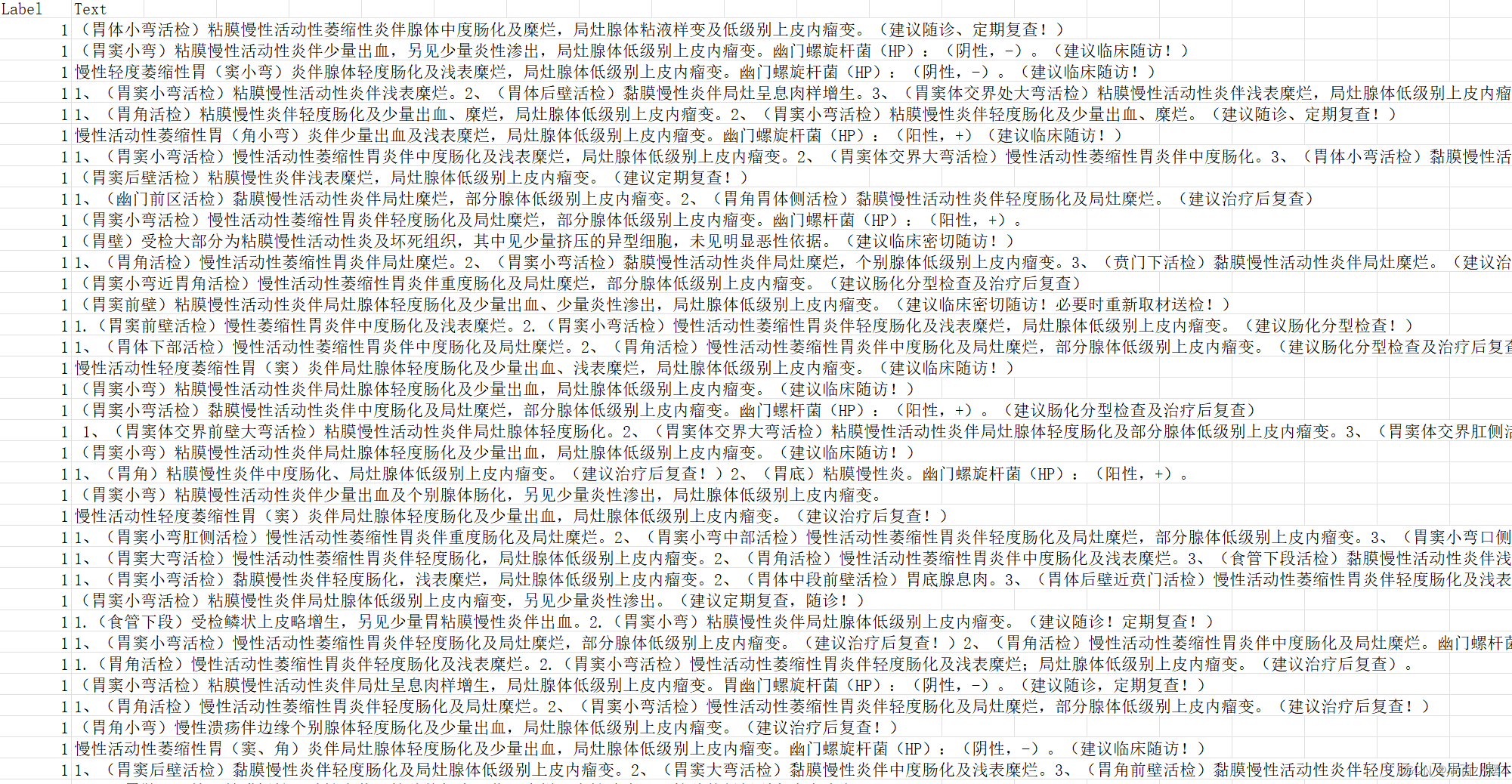
随着深度学习技术的发展，文本分类任务有了更加先进和精确的算法。除了传统的基于特征工程和机器学习算法的方法外，深度学习模型如卷积神经网络（CNN）、循环神经网络（RNN）、长短期记忆网络（LSTM）等也被广泛应用于文本分类。

TextCNN网络模型

TextCNN简介

TextCNN是一种用于文本分类的卷积神经网络模型。它主要应用于处理文本数据，如情感分析、垃圾邮件识别等任务。

TextCNN使用卷积神经网络的思想来处理文本数据。提到卷积神经网络，我们第一个想到的往往是对图像的特征提取，而TextCNN对文本词向量进行卷积提取特征是非常有创造性的。它的输入是一个句子或一个文本，通常通过将文本转换为词向量或字符向量的形式来表示。这些向量作为模型的输入，经过卷积层和池化层的处理，用于提取句子中的局部特征。然后将特征进行合并，并通过全连接层进行分类。

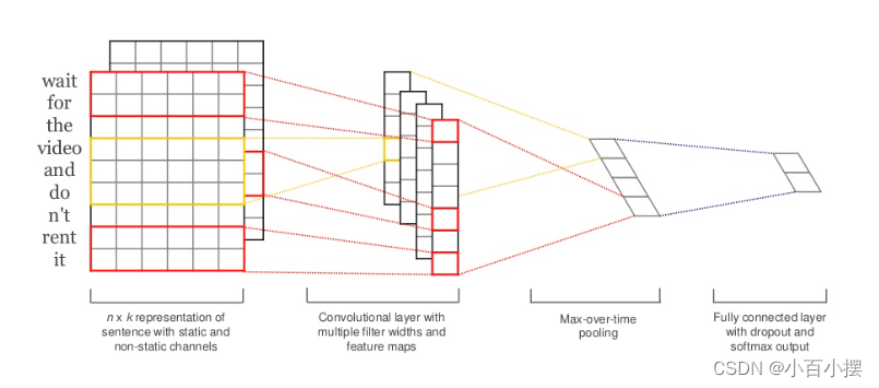
图1  TextCNN网络结构

TextCNN网络的处理流程如上图所示，首先是将输入的文本编码为固定长度的词向量或字符向量表示。再使用不同大小的卷积核在文本上进行卷积操作，在本文中我使用了[3,4,5]*词向量长度的不同卷积核大小，捕捉到不同尺寸的局部特征。卷积操作后进行池化，TextCNN的池化层对卷积层的输出进行最大池化，进一步减少特征数量，保留最重要的特征。最后经过全连接进行参数的学习，将池化层输出的特征向量连接到全连接层，并通过softmax作为损失函数进行分类。

TextCNN的优点是简单、高效，并且能够利用卷积神经网络在处理图像数据方面的成功经验来处理文本数据，同时在文本分类任务上取得不错的性能。

TextCNN对附件gastric.xlsx的分类处理

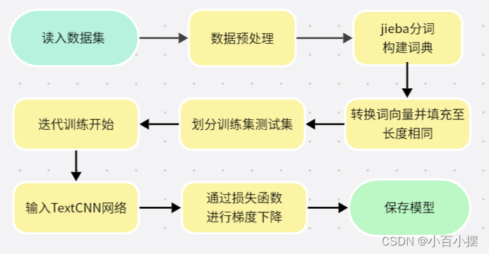
图2  本文中TextCNN处理流程

代码处理流程：首先通过pandas库读入gastric.xlsx数据集，并进行数据预处理，将文本内容和标签分别存储在变量中，接着使用jieba分词对文本进行分词处理，并构建词典，将每个词转换成对应的索引，以便后续用于构建词向量。将文本转换成词向量，并对文本进行填充，使得每个文本向量长度相同。之后划分训练集和测试集，并定义了TextCNN的文本分类模型，使用了Embedding层和多个卷积层进行特征提取，并利用池化层和全连接层进行五分类。再然后定义交叉熵损失函数、Adam优化器，创建数据加载器用于模型训练。进行模型训练，并记录每个epoch的训练损失和准确率，使用matplotlib库可视化训练过程中的损失和准确率变化，（采取的详细网络结构在代码附录中）。

TextCNN对附件gastric.xlsx的分类结果

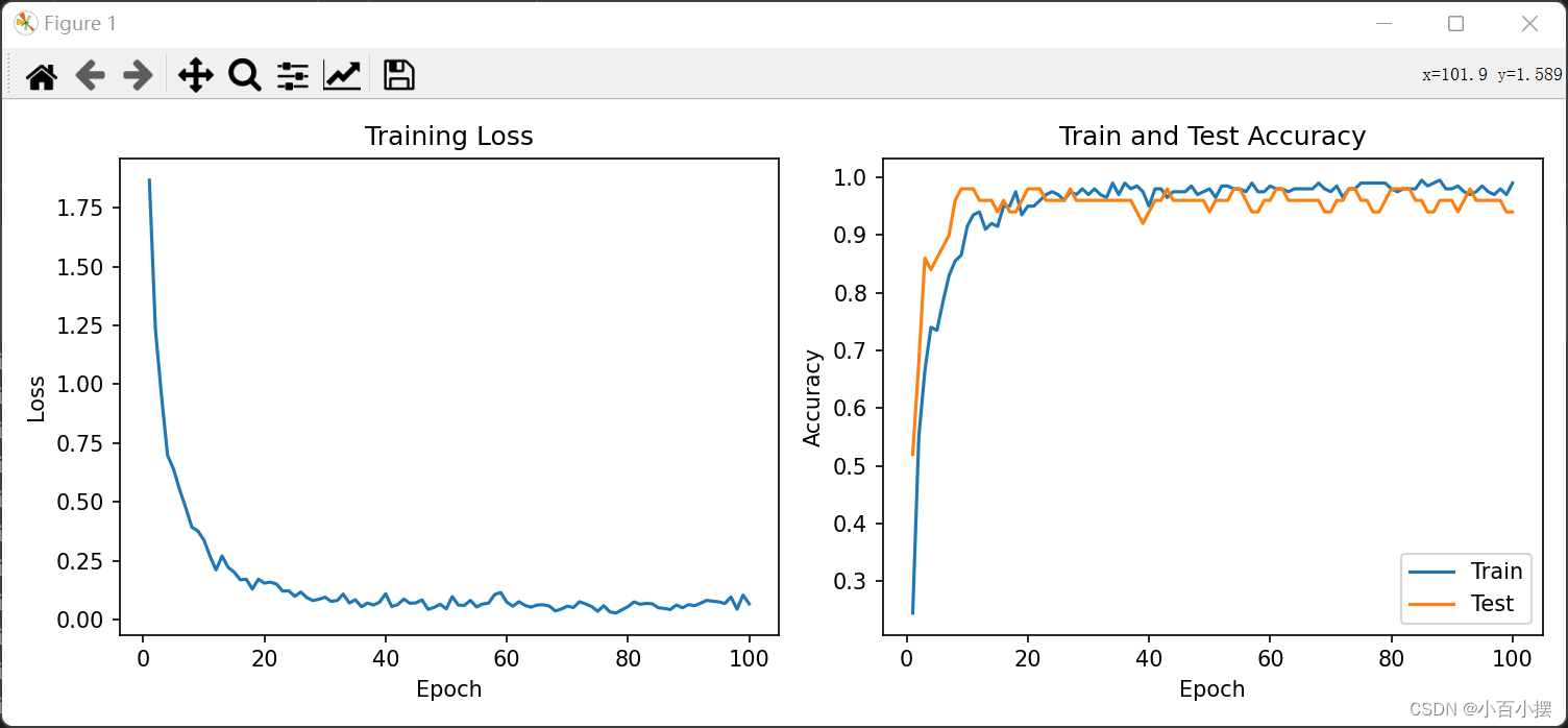
图3  TextCNN对gastric.xlsx数据集训练可视化

TextCNN分类任务对应各项指标为：

表1  TextCNN网络对gastric数据集分类性能各项指标

模型	准确率	精确率	召回率	F1
TextCNN	0.9400	0.9503	0.9520	0.9511

模型准确率和召回率都很高，并且F1值接近1，所以可以说模型在gastric数据集的文本分类任务上表现出很好的性能。模型能够准确地预测文本的类别，并且能够捕捉大多数文本分类的情况。对于250个数据样本的数据集，TextCNN是一个轻量级的深度学习网络，从训练集和测试集上准确率曲线的比较可以看到TextCNN在该数据集上也并没有表现出明显过拟合的问题。同时在训练次数为30次时，模型已经达到收敛，且正确率较高，近似取得了最佳参数。

TextRNN网络模型                                                                 

 TextRNN简介

TextRNN是一种基于循环神经网络（RNN）的文本分类模型。当处理文本数据时，TextRNN网络的循环神经网络结构使得模型能够捕捉到文本序列中的上下文信息。TextRNN通过逐步处理输入文本的每个词，并在每个时间步将当前词的向量表示和上一个时间步的隐藏状态作为输入，然后更新隐藏状态，并将其传递到下一个时间步。这种迭代的方式使得模型能够在处理整个文本序列时保留和利用历史信息。

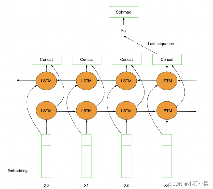
图4  TextRNN网络结构

在每个时间步，TextRNN模型可以使用多种循环神经网络结构，如基于门控循环单元（GRU）或长短期记忆（LSTM）的网络单元。这些网络单元具有记忆功能，能够有效处理长依赖关系。

在训练过程中，TextRNN模型与TextCNN模型相同，通常以词向量作为输入。（代表两种网络的数据预处理几乎一致），词向量我们可以通过预训练的词嵌入模型（如Word2Vec、GloVe等）得到，也可以在训练文本分类模型时与其他参数一同进行学习。

对于文本分类任务，TextRNN在模型的最后一个时间步上的隐藏状态，或者是整个序列的隐藏状态进行汇总。然后，可以将汇总的隐藏状态通过全连接层或其他分类器进行分类预测。

TextRNN的应用非常广泛。在情感分析中，模型可以通过学习句子的上下文信息，自动判断句子的情感倾向，如正面、负面或中性。另外，TextRNN也可以用于主题分类，将文本数据映射到特定的主题类别中。此外，TextRNN还可用于生成文本、机器翻译和问答系统等其他自然语言处理任务。

TextRNN同样是文本分类的经典深度学习算法。在文本分类问题上有很好的性能。

TextRNN对附件gastric.xlsx的分类处理

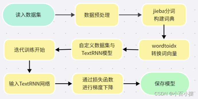
图5  本文中TextRNN处理流程（与TextCNN基本一致）

代码处理流程：我们的目的是使用TextRNN模型训练gastric数据集文本分类器。首先，导入需要使用的库，包括pandas用于读取数据集，jieba用于中文分词，torch用于构建和训练模型，matplotlib用于绘制损失和准确率的图表。

接下来读取数据集，使用pandas将文本和标签分别存储在texts和labels列表中。然后对文本进行分词处理，使用jieba库的lcut函数对每个文本进行分词，并使用空格连接各个词语，最后将结果存储在texts列表中。构建词向量，使用word2idx字典将词语映射为索引，并保存在列表中。然后创建自定义数据集TextClassificationDataset，继承了torch的Dataset类，重载了__len__和__getitem__方法，用于返回数据集的长度和指定索引位置的数据。

定义我们拟采用的TextRNN模型，使用nn.Embedding对词语进行编码，使用nn.RNN进行序列建模，最后通过全连接层进行五分类。确定超参数，然后是训练模型。使用了交叉熵损失函数和Adam优化器，在每个epoch中对训练集进行迭代训练，计算并记录损失和准确率。最后创建了数据加载器DataLoader，用于加载训练数据集，初始化了模型和优化器，调用函数进行模型训练。(采用的TextRNN具体网络结构在附录中)。

 TextRNN对附件gastric.xlsx的分类结果

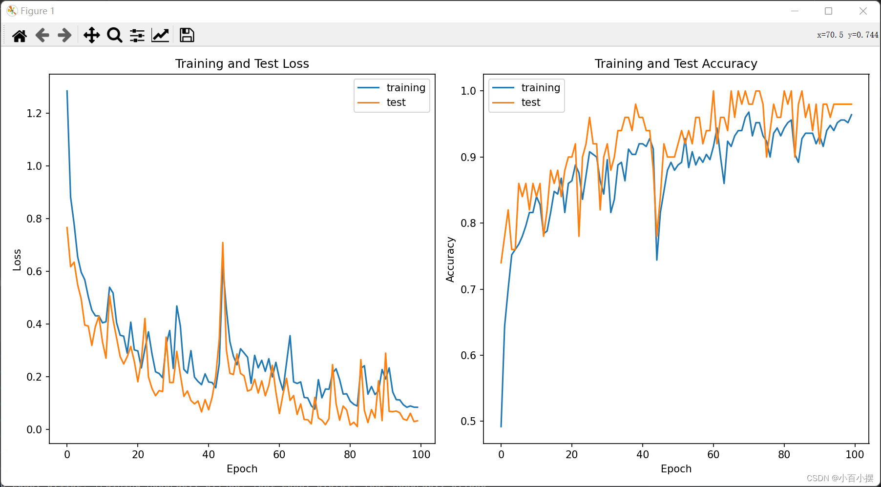
图6  TextRNN对gastric.xlsx数据集训练可视化

TextRNN分类任务对应各项指标为：

表2  TextRNN网络对gastric数据集分类性能各项指标

模型	准确率	精确率	召回率	F1
TextRNN	0.9833	0.9800	0.9800	0.9805

TextRNN模型的准确率和召回率同样都较高，在gastric数据集的文本分类任务上表现出不错的性能。在训练过程中体现的欠拟合虽然不是很明显，但还是有一定程度上的欠拟合且模型在训练100轮次后还是没有明显收敛，可能是由于样本容量为250的数据集对于循环神经网络这类参数较多的网络是不够的，但是TextRNN总体上来说还是取得了不错的效果。

其他深度学习算法

在这一模块列举一些常见的用于文本分类的深度学习算法，作为内容的补充拓展。

Transformers模型是一种基于自注意力机制（self-attention）的模型，广泛应用于自然语言处理任务。它具有较长的上下文关注和捕捉序列内部依赖关系的能力，适用于文本分类任务。ChatGPT就是基于Transformers架构预训练的大语言模型。

LSTM与GRU是除了TextRNN外，较为常用的循环神经网络模型，适用于处理序列数据。它们具有记忆单元和门控机制，能够较好地捕捉长距离的依赖关系，在文本分类中也得到了广泛的应用。

BERT是一种基于Transformer架构预训练的语言模型，利用大规模的无标签数据进行训练。BERT模型在各种自然语言处理任务中表现出色，并在文本分类中也取得了很好的效果。

FastText是由Facebook AI Research提出的文本分类工具，它利用了字符n-gram特征和高效的分类器。相较于传统基于词语的方法，FastText采用了基于字符的子词特征表示，能够处理未登录词并具有一定的泛化能力。FastText的训练和推理速度非常快，适用于处理大规模数据集和实时系统。它在文本分类任务中表现出色，特别适用于大数据集和较短的文本分类。

 结果分析与讨论

在完成文本分类任务方面，朴素贝叶斯和支持向量机等传统机器学习算法在速度和效果上表现良好，针对附件的文本分类正确率也能维持在70%左右。这些算法在处理较为简单的文本分类任务时较为适用。

然而，当面临更加复杂的文本分类任务时，传统机器学习算法的性能可能会受到限制。这是因为传统的一些机器学习算法难以捕捉文本中的复杂关系和上下文信息。相比之下，深度学习算法如TextCNN和TextRNN在处理复杂关系方面表现更加出色。TextCNN通过卷积层和池化层来捕捉文本中的局部特征，而TextRNN则通过递归神经网络来捕捉文本的序列信息，这使得它们能够更好地理解文本数据中的情感和上下文信息。

此外，深度学习算法在面对大规模数据集和自然语言处理领域的任务时，具有更高的准确性。深度学习模型通常由许多隐藏层组成，能够学习更多抽象和复杂的特征表示。因此，在处理需要更高准确性和对大规模数据集进行分类的文本任务时，深度学习算法通常是更好的选择。

表3  本文讨论的各模型/算法对gastric数据集分类性能各项指标

模型/算法	准确率	精确率	召回率	F1
SVM	0.72	0.72	0.71	0.69
朴素贝叶斯	0.68	0.75	0.68	0.66
TextCNN	0.94	0.95	0.95	0.95
TextRNN	0.98	0.98	0.98	0.98

注：上表中SVM使用的是TF-IDF，朴素贝叶斯使用的是词袋特征，均为最佳表现。

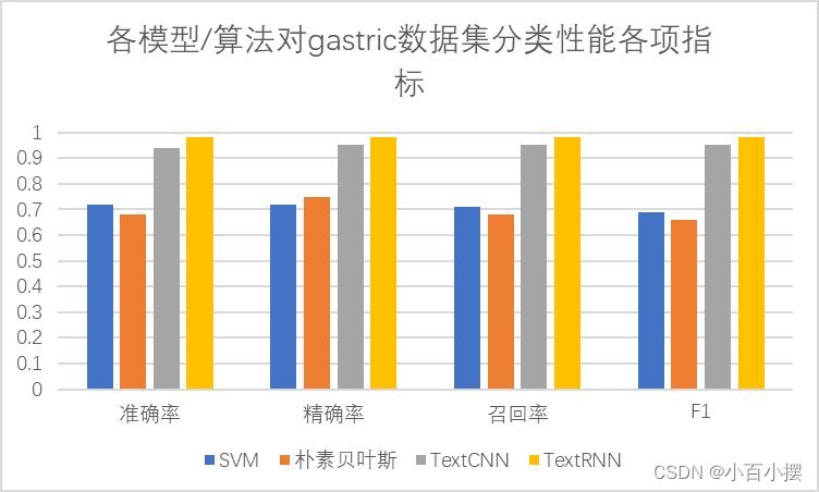
图7  可视化各模型/算法对gastric数据集分类性能各项指标

结合实验数据与上述讨论，针对文本分类任务，选择合适的机器学习和深度学习算法是至关重要的，它可以帮助提高分类的准确度和处理速度。对于简单的文本分类任务，传统的机器学习算法可能足够。而对于复杂的文本关系和大规模数据集，深度学习算法会更加适合并取得更好的效果。

附录：

TextCNN:

import pandas as pd
import jieba
import torch
import torch.nn as nn
import torch.optim as optim
from matplotlib import pyplot as plt
from torch.utils.data import TensorDataset, DataLoader
from sklearn.model_selection import train_test_split
from sklearn.metrics import precision_score, recall_score, f1_score, accuracy_score

# 读入数据集
data = pd.read_excel('../gastric.xlsx')
x = data['Text'].tolist()
y = data['Label'].tolist()


# 分词
def cut_text(text):
    return jieba.lcut(text)


x = [cut_text(text) for text in x]
print(x)

# 构建词典
word_count = {}
for text in x:
    for word in text:
        if word in word_count:
            word_count[word] += 1
        else:
            word_count[word] = 1
vocab = sorted(word_count, key=word_count.get, reverse=True)
word_to_index = {word: i + 2 for i, word in enumerate(vocab)}
word_to_index['<PAD>'] = 0
word_to_index['<UNK>'] = 1


# 将文本转换成词向量
def text_to_vector(text):
    return [word_to_index.get(word, 1) for word in text]


x = [text_to_vector(text) for text in x]

max_length = max(len(text) for text in x)
x = torch.tensor([text + [0] * (max_length - len(text)) for text in x])
y = torch.tensor(y)

x_train, x_test, y_train, y_test = train_test_split(x, y, test_size=0.2)


class TextCNN(nn.Module):
    def __init__(self, vocab_size, embedding_dim, output_dim, n_filters, filter_sizes, dropout):
        super().__init__()
        self.embedding = nn.Embedding(vocab_size, embedding_dim)
        self.conv_layers = nn.ModuleList([
            nn.Conv1d(in_channels=embedding_dim,
                      out_channels=n_filters,
                      kernel_size=fs)
            for fs in filter_sizes
        ])
        self.fc = nn.Linear(n_filters * len(filter_sizes), output_dim)
        self.dropout = nn.Dropout(dropout)

    def forward(self, text):
        embedded = self.embedding(text)
        embedded = embedded.permute(0, 2, 1)
        conved = [nn.functional.relu(conv(embedded)) for conv in self.conv_layers]
        pooled = [nn.functional.max_pool1d(conv, conv.shape[2]).squeeze(2) for conv in conved]
        cat = self.dropout(torch.cat(pooled, dim=1))
        output = self.fc(cat)
        return output


batch_size = 64
learning_rate = 0.001
num_epochs = 100
vocab_size = len(word_to_index)
embedding_dim = 100
output_dim = 6
n_filters = 100
filter_sizes = [3, 4, 5]
dropout = 0.5

model = TextCNN(vocab_size, embedding_dim, output_dim, n_filters, filter_sizes, dropout)
criterion = nn.CrossEntropyLoss()
optimizer = optim.Adam(model.parameters(), lr=learning_rate)

train_ds = TensorDataset(x_train, y_train)
train_loader = DataLoader(train_ds, batch_size=batch_size, shuffle=True)

train_loss_history = []
train_acc_history = []
test_acc_history = []

for epoch in range(num_epochs):
    train_loss = 0.0
    total_samples = 0
    correct_samples = 0

    model.train()
    for x_batch, y_batch in train_loader:
        optimizer.zero_grad()
        outputs = model(x_batch)
        loss = criterion(outputs, y_batch)
        loss.backward()
        optimizer.step()

        train_loss += loss.item() * x_batch.size(0)
        total_samples += x_batch.size(0)
        correct_samples += (torch.argmax(outputs, dim=1) == y_batch).sum().item()

    train_loss /= total_samples
    train_acc = correct_samples / total_samples
    train_loss_history.append(train_loss)
    train_acc_history.append(train_acc)

    with torch.no_grad():
        model.eval()
        y_pred = model(x_test)
        y_pred = torch.argmax(y_pred, dim=1)
        test_acc = (y_pred == y_test).sum().item() / len(y_test)
        test_acc_history.append(test_acc)

    print(
        f'Epoch [{epoch + 1}/{num_epochs}], Loss: {train_loss:.4f}, Train Accuracy: {train_acc:.4f}, Test Accuracy: {test_acc:.4f}')

# 可视化训练过程
plt.figure(figsize=(10, 4))
plt.subplot(1, 2, 1)
plt.plot(range(1, num_epochs + 1), train_loss_history)
plt.xlabel('Epoch')
plt.ylabel('Loss')
plt.title('Training Loss')

plt.subplot(1, 2, 2)
plt.plot(range(1, num_epochs + 1), train_acc_history, label='Train')
plt.plot(range(1, num_epochs + 1), test_acc_history, label='Test')
plt.xlabel('Epoch')
plt.ylabel('Accuracy')
plt.title('Train and Test Accuracy')
plt.legend()

plt.tight_layout()
plt.show()

# 获取测试集上的预测结果
model.eval()
y_pred = model(x_test)
y_pred = torch.argmax(y_pred, dim=1).tolist()
y_test = y_test.tolist()

# 计算准确率
accuracy = accuracy_score(y_test, y_pred)
# 计算召回率
recall = recall_score(y_test, y_pred, average='macro')
# 计算F1值
f1 = f1_score(y_test, y_pred, average='macro')
# 计算精确率
precision = precision_score(y_test, y_pred, average='macro')

# 打印结果
print("准确率：%.4f" % accuracy)
print("召回率：%.4f" % recall)
print("F1值：%.4f" % f1)
print("精确率：%.4f" % precision)

TextRNN:

import pandas as pd
import jieba
import torch
import torch.nn as nn
import torch.optim as optim
from torch.utils.data import Dataset, DataLoader
import matplotlib.pyplot as plt
from sklearn.metrics import accuracy_score, precision_score, recall_score, f1_score

# 读取数据集
data = pd.read_excel('../gastric.xlsx')
texts = data['Text'].tolist()
labels = data['Label'].tolist()

# 分词
texts = [' '.join(jieba.lcut(text)) for text in texts]

# 构建词向量
word2idx = {}
idx = 0
for text in texts:
    for word in text.split():
        if word not in word2idx:
            word2idx[word] = idx
            idx += 1

# 构建数据集
word_indices = [[word2idx[word] for word in text.split()] for text in texts]
label_indices = [int(label) for label in labels]


# 定义自定义数据集
class TextClassificationDataset(Dataset):
    def __init__(self, word_indices, label_indices):
        self.word_indices = word_indices
        self.label_indices = label_indices

    def __len__(self):
        return len(self.word_indices)

    def __getitem__(self, idx):
        return torch.tensor(self.word_indices[idx]), torch.tensor(self.label_indices[idx])


# 初始化模型参数
vocab_size = len(word2idx)
embedding_dim = 100
hidden_dim = 128
num_classes = 6
learning_rate = 0.001
num_epochs = 100


# 定义RNN模型
class RNN(nn.Module):
    def __init__(self, vocab_size, embedding_dim, hidden_dim, num_classes):
        super(RNN, self).__init__()
        self.embedding = nn.Embedding(vocab_size, embedding_dim)
        self.rnn = nn.RNN(embedding_dim, hidden_dim, batch_first=True)
        self.fc = nn.Linear(hidden_dim, num_classes)

    def forward(self, x):
        embeds = self.embedding(x)
        out, _ = self.rnn(embeds)
        out = self.fc(out[:, -1, :])
        return out


# 训练模型
def train_model(model, criterion, optimizer, train_loader, num_epochs):
    loss_history = []
    accuracy_history = []
    test_loss_history = []
    test_accuracy_history = []

    for epoch in range(num_epochs):
        total_loss = 0
        correct = 0
        total_samples = 0

        test_total_loss = 0
        test_correct = 0
        test_total_samples = 0

        for inputs, labels in train_loader:
            optimizer.zero_grad()
            outputs = model(inputs)
            loss = criterion(outputs, labels)
            loss.backward()
            optimizer.step()
            total_loss += loss.item()

            _, predicted = torch.max(outputs, 1)
            correct += (predicted == labels).sum().item()
            total_samples += labels.size(0)

        # 在测试集上评估模型
        with torch.no_grad():
            for test_inputs, test_labels in test_loader:
                test_outputs = model(test_inputs)
                test_loss = criterion(test_outputs, test_labels)
                test_total_loss += test_loss.item()

                _, test_predicted = torch.max(test_outputs, 1)
                test_correct += (test_predicted == test_labels).sum().item()
                test_total_samples += test_labels.size(0)

        epoch_loss = total_loss / len(train_loader)
        epoch_accuracy = correct / total_samples
        test_epoch_loss = test_total_loss / len(test_loader)
        test_epoch_accuracy = test_correct / test_total_samples

        loss_history.append(epoch_loss)
        accuracy_history.append(epoch_accuracy)
        test_loss_history.append(test_epoch_loss)
        test_accuracy_history.append(test_epoch_accuracy)
        print(f'Epoch {epoch + 1}/{num_epochs}, '
              f'Training Loss: {epoch_loss:.4f}, Training Accuracy: {epoch_accuracy:.4f}, '
              f'Test Loss: {test_epoch_loss:.4f}, Test Accuracy: {test_epoch_accuracy:.4f}')

    # 绘制训练和测试的损失和正确率曲线
    plt.figure(figsize=(12, 6))
    plt.subplot(1, 2, 1)
    plt.plot(loss_history, label='training')
    plt.plot(test_loss_history, label='test')
    plt.xlabel('Epoch')
    plt.ylabel('Loss')
    plt.title('Training and Test Loss')
    plt.legend()

    plt.subplot(1, 2, 2)
    plt.plot(accuracy_history, label='training')
    plt.plot(test_accuracy_history, label='test')
    plt.xlabel('Epoch')
    plt.ylabel('Accuracy')
    plt.title('Training and Test Accuracy')
    plt.legend()

    plt.tight_layout()
    plt.show()


# 创建数据加载器
dataset = TextClassificationDataset(word_indices, label_indices)
train_loader = DataLoader(dataset, batch_size=1, shuffle=True)

# 初始化模型和优化器
model = RNN(vocab_size, embedding_dim, hidden_dim, num_classes)
optimizer = optim.Adam(model.parameters(), lr=learning_rate)
criterion = nn.CrossEntropyLoss()

# 分割数据集为训练集和测试集
train_size = int(0.8 * len(dataset))
test_size = len(dataset) - train_size
train_dataset, test_dataset = torch.utils.data.random_split(dataset, [train_size, test_size])

# 创建测试集加载器
test_loader = DataLoader(test_dataset, batch_size=1, shuffle=True)

# 训练模型
train_model(model, criterion, optimizer, train_loader, num_epochs)

# 在测试集上进行预测
y_true = []
y_pred = []
with torch.no_grad():
    for inputs, labels in test_loader:
        outputs = model(inputs)
        _, predicted = torch.max(outputs, 1)
        y_true.extend(labels.numpy())
        y_pred.extend(predicted.numpy())

# 计算评估指标
f1 = f1_score(y_true, y_pred, average='weighted')
precision = precision_score(y_true, y_pred, average='weighted')
recall = recall_score(y_true, y_pred, average='weighted')
accuracy = accuracy_score(y_true, y_pred)

print(f'F1: {f1:.4f}, Precision: {precision:.4f}, Recall: {recall:.4f}, Accuracy: {accuracy:.4f}')