机器学习6：单层感知器

机器学习6：单层感知器

单层感知器

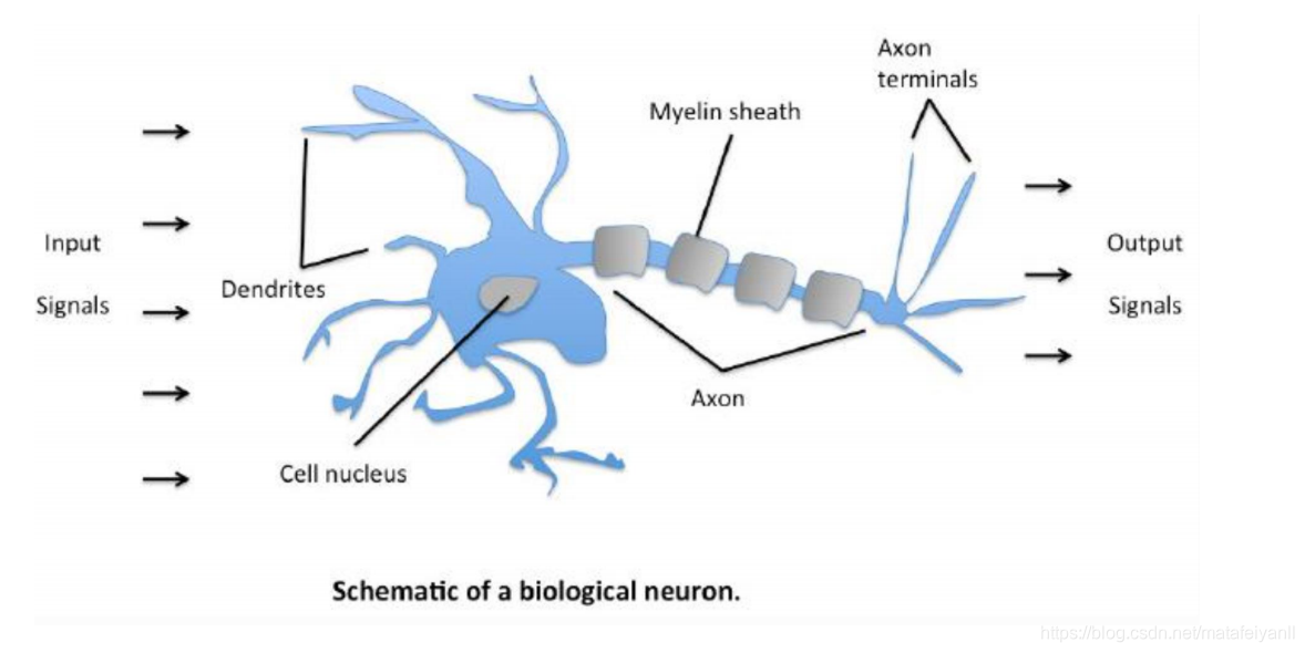
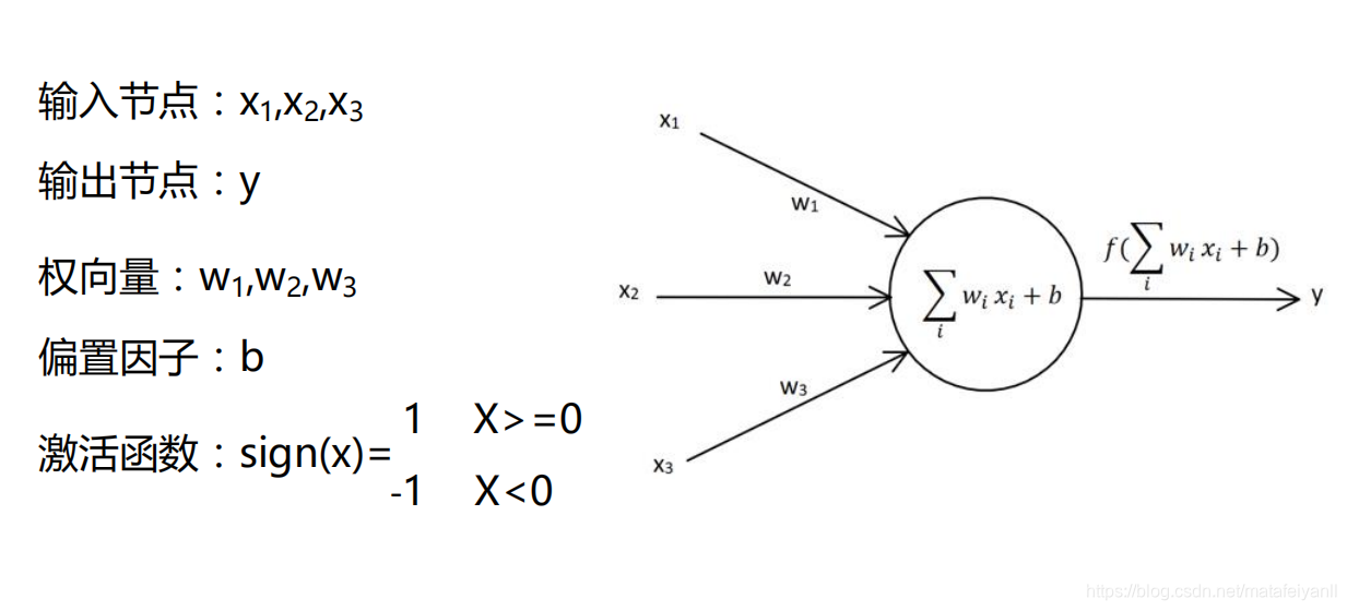
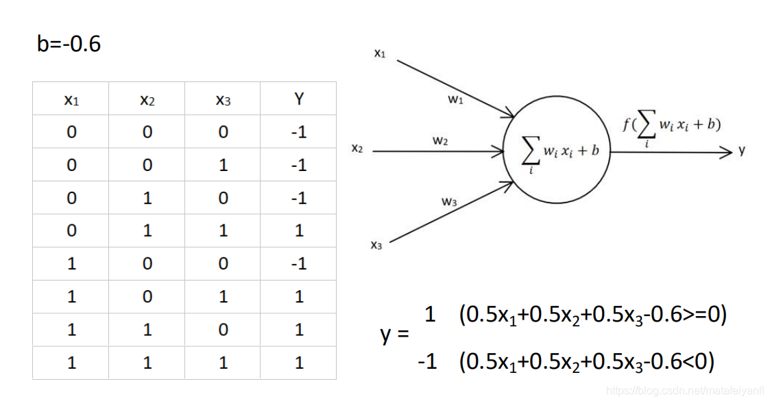
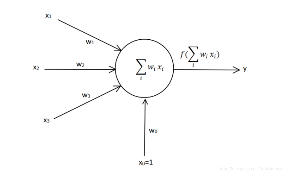
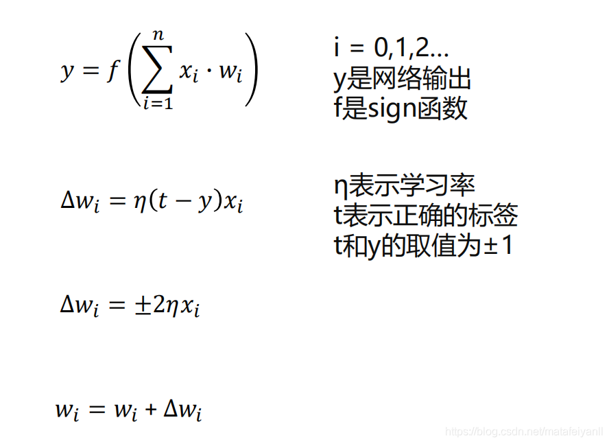
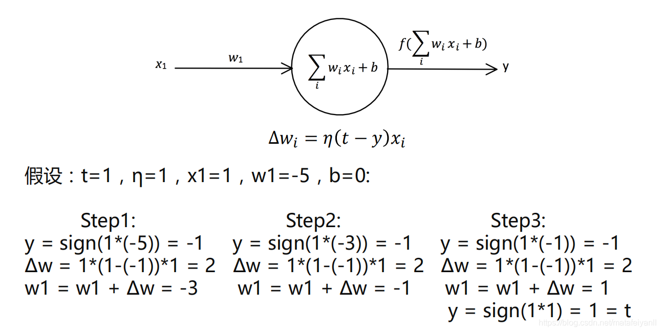
原理

感知器学习规则

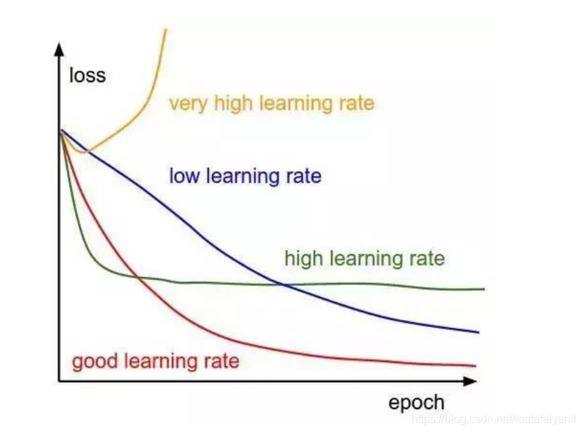
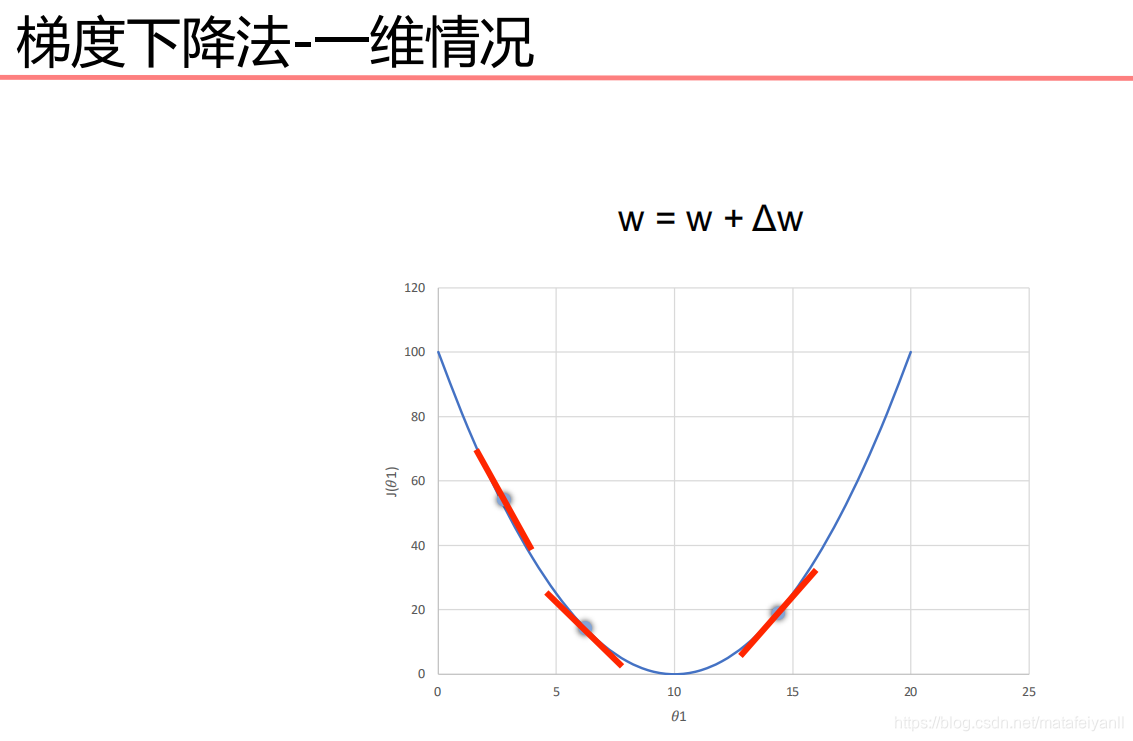
关于学习率

𝜂取值一般取0-1之间
学习率太大容易造成权值调整不稳定
学习率太小，权值调整太慢，迭代次数太多

模型收敛条件
误差小于某个预先设定的较小的值
两次迭代之间的权值变化已经很小
设定最大迭代次数，当迭代超过最大次数就停止

线性神经网络

线性神经网络在结构上与感知器非常相似，只是激活函数不同。
在模型训练时把原来的sign函数改成了purelin函数：y = x
关于激活函数

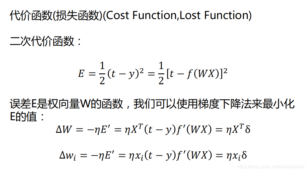
Delta学习规则

算法实现

简单的单层感知器

import numpy as np
import matplotlib.pyplot as plt

#载入数据
X=np.array([[1,3,3],
           [1,4,3],
           [1,1,1],
           [1,0,2]])
#标签
Y=np.array([[1],
           [1],
           [-1],
           [-1]])
#权值初始化 ，3个输入，1个输出，3行1列，取值范围-1~1,本身取值范围为0~1
W=(np.random.random([3,1])-0.5)*2
print(W)

#设置学习率
lr=0.11
#神经网络输出
O=1

#权值更新
def update():
    global X,Y,W,lr
    O=np.sign(np.dot(X,W))  
    W_C=lr*(X.T.dot(Y-O))/int(X.shape[0])
    W=W+W_C

[[ 0.68420477]
[ 0.25176422]
[-0.38435113]]

for i in range(100):
    update()   #更新权值
    print(W)   #打印权值
    print(i)  #打印当前迭代次数
    O=np.sign(np.dot(X,W))  #计算当前输出
    if(O==Y).all():
        print("Finished")
        print("epoch:",i)
        break
        
#正样本
x1=[3,4]
y1=[3,3]
#负样本
x2=[1,0]
y2=[1,2]

#计算分界线的斜率以及截距
k=-W[1]/W[2]
d=-W[0]/W[2]
print('k=',k)
print('d=',d)

xdata=(0,5)

plt.figure()
plt.plot(xdata,xdata*k+d,'r')
plt.scatter(x1,y1,c='b')
plt.scatter(x2,y2,c='r')
plt.show()

线性感知器

import numpy as np
import matplotlib.pyplot as plt

#输入数据
X = np.array([[1,3,3],
              [1,4,3],
              [1,1,1],
              [1,0,2]])
#标签
Y = np.array([[1],
              [1],
              [-1],
              [-1]])

#权值初始化，3行1列，取值范围-1到1
W = (np.random.random([3,1])-0.5)*2

print(W)
#学习率设置
lr = 0.11
#神经网络输出
O = 0

def update():
    global X,Y,W,lr
    O = np.dot(X,W)  #y=x线性激活函数
    W_C = lr*(X.T.dot(Y-O))/int(X.shape[0])
    W = W + W_C


for _ in range(1000):
    update()#更新权值

    #正样本
    x1 = [3,4]
    y1 = [3,3]
    #负样本
    x2 = [1,0]
    y2 = [1,2]

    #计算分界线的斜率以及截距
    k = -W[1]/W[2]
    d = -W[0]/W[2]
    print('k=',k)
    print('d=',d)

    xdata = (0,5)

    plt.figure()
    plt.plot(xdata,xdata*k+d,'r')
    plt.scatter(x1,y1,c='b')
    plt.scatter(x2,y2,c='y')
    plt.show()

线性感知器不能解决异或问题

‘’’
异或
0^0 = 0
0^1 = 1
1^0 = 1
1^1 = 0
‘’’

找不到一条直线将两个类分开

异或问题的解决

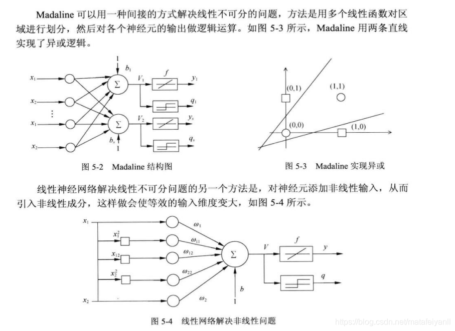
这里采用引入非线性输入

import numpy as np
import matplotlib.pyplot as plt

#输入数据
X = np.array([[1,0,0,0,0,0],
              [1,0,1,0,0,1],
              [1,1,0,1,0,0],
              [1,1,1,1,1,1]])
#标签
Y = np.array([[-1],
              [1],
              [1],
              [-1]])

#权值初始化，3行1列，取值范围-1到1
W = (np.random.random([6,1])-0.5)*2
print(W)

#学习率设置
lr = 0.11
#计算迭代次数
n = 0
#神经网络输出
O = 0

def update():
    global X,Y,W,lr,n
    n+=1
    O = np.dot(X,W)  #y=x线性激活函数
    W_C = lr*(X.T.dot(Y-O))/int(X.shape[0])
    W = W + W_C

[[-0.25710504]
[ 0.43289465]
[-0.02744922]
[ 0.50894635]
[ 0.96606606]
[-0.91572789]]

for _ in range(1000):
    update()#更新权值
    
#正样本
x1 = [0,1]
y1 = [1,0]
#负样本
x2 = [0,1]
y2 = [0,1]


#画图，计算x2的值，root=1返回正根
def calculate(x,root):
    a=W[5]
    b=W[2]+W[4]*x
    c=W[1]*x+W[3]*x*x+W[0]
    if(root==1):
        return((-b+np.sqrt(b*b-4*a*c))/2/a)
    if(root==0):
        return((-b-np.sqrt(b*b-4*a*c))/2/a)
    

xdata = np.linspace(0,1)

plt.figure()

plt.plot(xdata,calculate(xdata,1),'r')
plt.plot(xdata,calculate(xdata,0),'r')
plt.plot(x1,y1,'bo')
plt.plot(x2,y2,'yo')

plt.show()