cs231深度学习课程，注意点总结

从今天开始，正式踏入深度学习的行列。之前接触过一些，但都不系统。这次从cs231课程开始。

Why Mini-batch gradient descent can work？？？

http://cs231n.github.io/optimization-1/

Mini-batch gradient descent. In large-scale applications (such as the ILSVRC challenge), the training data can have on order of millions of examples. Hence, it seems wasteful to compute the full loss function over the entire training set in order to perform only a single parameter update. A very common approach to addressing this challenge is to compute the gradient over batches of the training data. For example, in current state of the art ConvNets, a typical batch contains 256 examples from the entire training set of 1.2 million. This batch is then used to perform a parameter update:

# Vanilla Minibatch Gradient Descent

while True:
  data_batch = sample_training_data(data, 256) # sample 256 examples
  weights_grad = evaluate_gradient(loss_fun, data_batch, weights)
  weights += - step_size * weights_grad # perform parameter update

The reason this works well is that the examples in the training data are correlated. To see this, consider the extreme case where all 1.2 million images in ILSVRC are in fact made up of exact duplicates of only 1000 unique images (one for each class, or in other words 1200 identical copies of each image). Then it is clear that the gradients we would compute for all 1200 identical copies would all be the same, and when we average the data loss over all 1.2 million images we would get the exact same loss as if we only evaluated on a small subset of 1000. In practice of course, the dataset would not contain duplicate images, the gradient from a mini-batch is a good approximation of the gradient of the full objective. Therefore, much faster convergence can be achieved in practice by evaluating the mini-batch gradients to perform more frequent parameter updates.

The extreme case of this is a setting where the mini-batch contains only a single example. This process is calledStochastic Gradient Descent (SGD) (or also sometimes on-line gradient descent). This is relatively less common to see because in practice due to vectorized code optimizations it can be computationally much more efficient to evaluate the gradient for 100 examples, than the gradient for one example 100 times. Even though SGD technically refers to using a single example at a time to evaluate the gradient, you will hear people use the term SGD even when referring to mini-batch gradient descent (i.e. mentions of MGD for “Minibatch Gradient Descent”, or BGD for “Batch gradient descent” are rare to see), where it is usually assumed that mini-batches are used. The size of the mini-batch is a hyperparameter but it is not very common to cross-validate it. It is usually based on memory constraints (if any), or set to some value, e.g. 32, 64 or 128. We use powers of 2 in practice because many vectorized operation implementations work faster when their inputs are sized in powers of 2.

three most commonly used gates in neural networks (add,mul,max)

http://cs231n.github.io/optimization-2/

It is interesting to note that in many cases the backward-flowing gradient can be interpreted on an intuitive level. For example, the three most commonly used gates in neural networks (add,mul,max), all have very simple interpretations in terms of how they act during backpropagation. Consider this example circuit:

Looking at the diagram above as an example, we can see that:

The add gate always takes the gradient on its output and distributes it equally to all of its inputs, regardless of what their values were during the forward pass. This follows from the fact that the local gradient for the add operation is simply +1.0, so the gradients on all inputs will exactly equal the gradients on the output because it will be multiplied by x1.0 (and remain unchanged). In the example circuit above, note that the + gate routed the gradient of 2.00 to both of its inputs, equally and unchanged.

The max gate routes the gradient. Unlike the add gate which distributed the gradient unchanged to all its inputs, the max gate distributes the gradient (unchanged) to exactly one of its inputs (the input that had the highest value during the forward pass). This is because the local gradient for a max gate is 1.0 for the highest value, and 0.0 for all other values. In the example circuit above, the max operation routed the gradient of 2.00 to the z variable, which had a higher value than w, and the gradient on w remains zero.

The multiply gate is a little less easy to interpret. Its local gradients are the input values (except switched), and this is multiplied by the gradient on its output during the chain rule. In the example above, the gradient on x is -8.00, which is -4.00 x 2.00.

Unintuitive effects and their consequences. Notice that if one of the inputs to the multiply gate is very small and the other is very big, then the multiply gate will do something slightly unintuitive: it will assign a relatively huge gradient to the small input and a tiny gradient to the large input.Note that in linear classifiers where the weights are dot producted  wTxi (multiplied) with the inputs, this implies that the scale of the data has an effect on the magnitude of the gradient for the weights. For example, if you multiplied all input data examples  xi  by 1000 during preprocessing, then the gradient on the weights will be 1000 times larger, and you’d have to lower the learning rate by that factor to compensate. This is why preprocessing matters a lot, sometimes in subtle ways! And having intuitive understanding for how the gradients flow can help you debug some of these cases.

interpretation of the gradient

The derivative on each variable tells you the sensitivity of the whole expression on its value.

Commonly used activation functions

介绍每个activation function的优缺点比较全面。

http://cs231n.github.io/neural-networks-1/

Every activation function (or non-linearity) takes a single number and performs a certain fixed mathematical operation on it. There are several activation functions you may encounter in practice:

 

Left: Sigmoid non-linearity squashes real numbers to range between [0,1]  Right: The tanh non-linearity squashes real numbers to range between [-1,1].

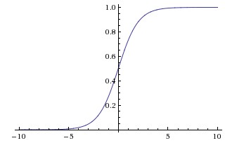
Sigmoid. The sigmoid non-linearity has the mathematical form  σ(x)=1/(1+e−x) σx11ex and is shown in the image above on the left. As alluded to in the previous section, it takes a real-valued number and “squashes” it into range between 0 and 1. In particular, large negative numbers become 0 and large positive numbers become 1. The sigmoid function has seen frequent use historically since it has a nice interpretation as the firing rate of a neuron: from not firing at all (0) to fully-saturated firing at an assumed maximum frequency (1).In practice, the sigmoid non-linearity has recently fallen out of favor and it is rarely ever used. It has two major drawbacks:

• Sigmoids saturate and kill gradients. A very undesirable property of the sigmoid neuron is that when the neuron’s activation saturates at either tail of 0 or 1, the gradient at these regions is almost zero. Recall that during backpropagation, this (local) gradient will be multiplied to the gradient of this gate’s output for the whole objective. Therefore, if the local gradient is very small, it will effectively “kill” the gradient and almost no signal will flow through the neuron to its weights and recursively to its data. Additionally, one must pay extra caution when initializing the weights of sigmoid neurons to prevent saturation. For example, if the initial weights are too large then most neurons would become saturated and the network will barely learn.
• Sigmoid outputs are not zero-centered. This is undesirable since neurons in later layers of processing in a Neural Network (more on this soon) would be receiving data that is not zero-centered. This has implications on the dynamics during gradient descent, because if the data coming into a neuron is always positive (e.g.  x>0 x0 elementwise in  f=wTx+b fwTxb)), then the gradient on the weights  w w will during backpropagation become either all be positive, or all negative (depending on the gradient of the whole expression  f f). This could introduce undesirable zig-zagging dynamics in the gradient updates for the weights. However, notice that once these gradients are added up across a batch of data the final update for the weights can have variable signs, somewhat mitigating this issue. Therefore, this is an inconvenience but it has less severe consequences compared to the saturated activation problem above.

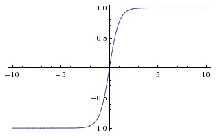
Tanh. The tanh non-linearity is shown on the image above on the right. It squashes a real-valued number to the range [-1, 1]. Like the sigmoid neuron, its activations saturate, but unlike the sigmoid neuron its output is zero-centered. Therefore, in practice the tanh non-linearity is always preferred to the sigmoid nonlinearity. Also note that the tanh neuron is simply a scaled sigmoid neuron, in particular the following holds:  tanh(x)=2σ(2x)−1 tanhx2σ2x1.

 

Left: Rectified Linear Unit (ReLU) activation function, which is zero when x &lt 0 and then linear with slope 1 when x &gt 0.  Right: A plot from  Krizhevsky et al. (pdf) paper indicating the 6x improvement in convergence with the ReLU unit compared to the tanh unit.

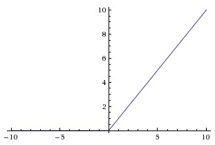
ReLU. The Rectified Linear Unit has become very popular in the last few years. It computes the function  f(x)=max(0,x) fx0x. In other words, the activation is simply thresholded at zero (see image above on the left). There are several pros and cons to using the ReLUs:

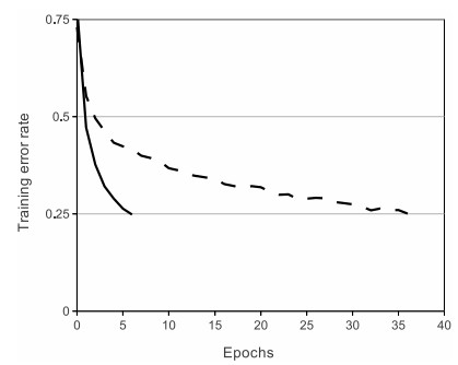
• (+) It was found to greatly accelerate (e.g. a factor of 6 in Krizhevsky et al.) the convergence of stochastic gradient descent compared to the sigmoid/tanh functions. It is argued that this is due to its linear, non-saturating form.
• (+) Compared to tanh/sigmoid neurons that involve expensive operations (exponentials, etc.), the ReLU can be implemented by simply thresholding a matrix of activations at zero.
• (-) Unfortunately, ReLU units can be fragile during training and can “die”. For example, a large gradient flowing through a ReLU neuron could cause the weights to update in such a way that the neuron will never activate on any datapoint again. If this happens, then the gradient flowing through the unit will forever be zero from that point on. That is, the ReLU units can irreversibly die during training since they can get knocked off the data manifold. For example, you may find that as much as 40% of your network can be “dead” (i.e. neurons that never activate across the entire training dataset) if the learning rate is set too high. With a proper setting of the learning rate this is less frequently an issue.

Leaky ReLU. Leaky ReLUs are one attempt to fix the “dying ReLU” problem. 自己看原文吧，老截断。