Stanford公开课机器学习---week3-1.Logistic Regression 逻辑回归

1 分类 Classification

在分类问题中,我们尝试预测的是结果是否属于某一个类(例如正确或错误)。
分类问题的例子有:

• 判断一封电子邮件是否是垃圾邮件;
• 判断一次金融交易是否是欺诈等等。

我们从二元的分类问题开始讨论。
我们将因变量(dependant variable)可能属于的两个类分别称为

• 负向类(negative class)，因变量 0 表示
• 正向类(positive class)，因变量 1 表示

Instead of our output vector y being a continuous range of values, it will only be 0 or 1.
y∈{0,1}
Where 0 is usually taken as the “negative class” and 1 as the “positive class”, but you are free to assign any representation to it.
We’re only doing two classes for now, called a “Binary Classification Problem.”
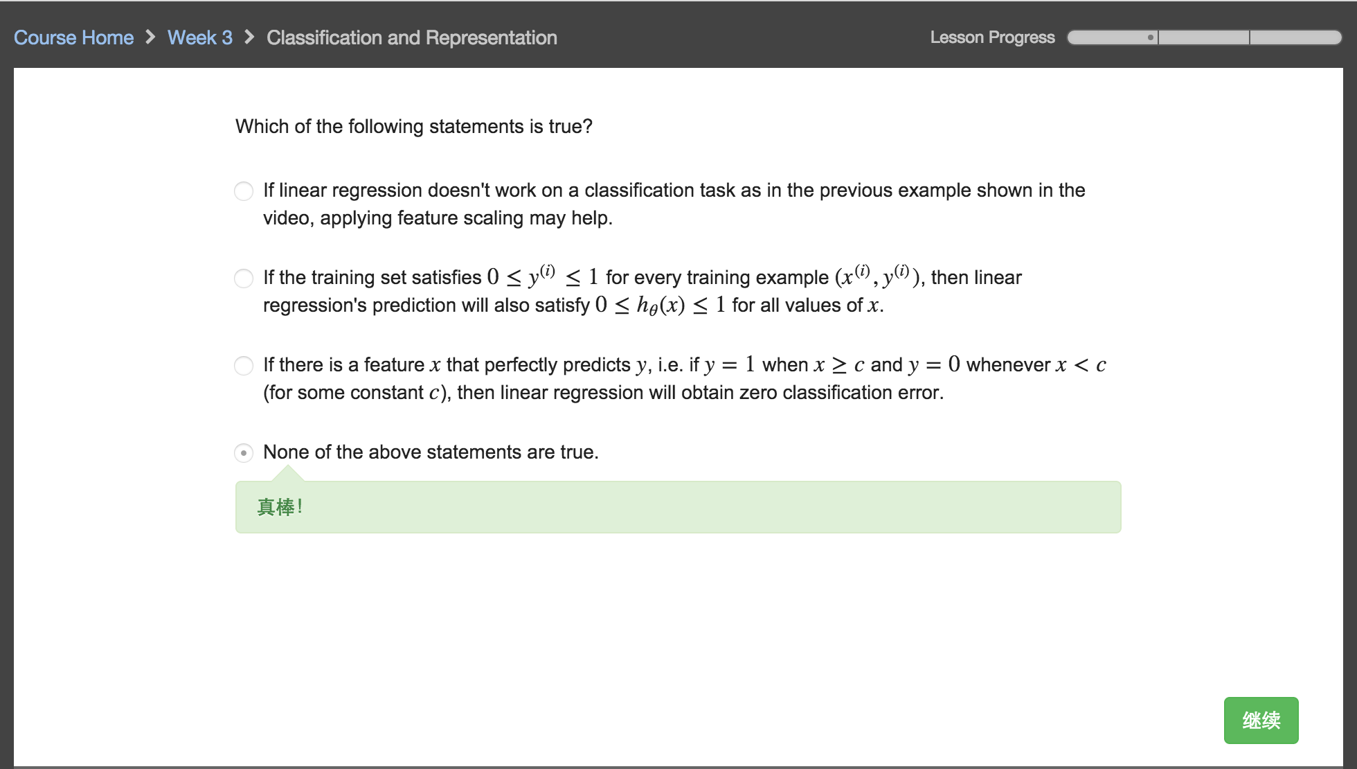
One method is to use linear regression and map all predictions greater than 0.5 as a 1 and all less than 0.5 as a 0. This method doesn’t work well because classification is not actually a linear function.

---

2 假设表示 Hypothesis Representation

乳腺癌分类问题,我们可以用线性回归的方法求出适合数据的一条直线:
根据线性回归模型我们只能预测连续的直,然而对于分类问题,我们需要输出 0 或 1,我们可以预测:

• 当 hθ大于等于 0.5 时,预测 y=1
• 当 hθ小于 0.5 时,预测 y=0

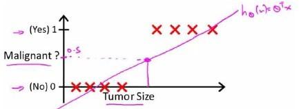
对于上图所示的数据,这样的一个线性模型似乎能很好地完成分类任务。假使我们又观测到一 个非常大尺寸的恶性肿瘤,将其作为实例加入到我们的训练集中来,这将使得我们获得一条新的直线。

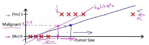
这时,再使用 0.5 作为阀值来预测肿瘤是良性还是恶性便不合适了。可以看出,线性回归模型, 因为其预测的值可以超越[0,1]的范围,并不适合解决这样的问题。

我们引入一个新的模型,逻辑回归,该模型的输出变量范围始终在 0 和 1 之间。 逻辑回归模型的假设是:

$$\large y \in \lbrace 0,1 \rbrace$$
$$\large \begin{align*} & h_\theta (x) = g ( \theta^T x ) \newline \newline & z = \theta^T x \newline & g(z) = \dfrac{1}{1 + e^{-z}} \end{align*}$$
其中:

• X 代表特征向量
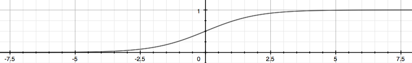
• g 代表逻辑函数(logistic function)是一个常用的逻辑函数为 S 形函数(Sigmoid function),公式为:$g(z) = \dfrac{1}{1 + e^{-z}}$
  

该函数的图像为:

合起来,我们得到逻辑回归模型的假设:

$$g(z) = \dfrac{1}{1 + e^{-\theta^T x }}$$

对模型的理解:

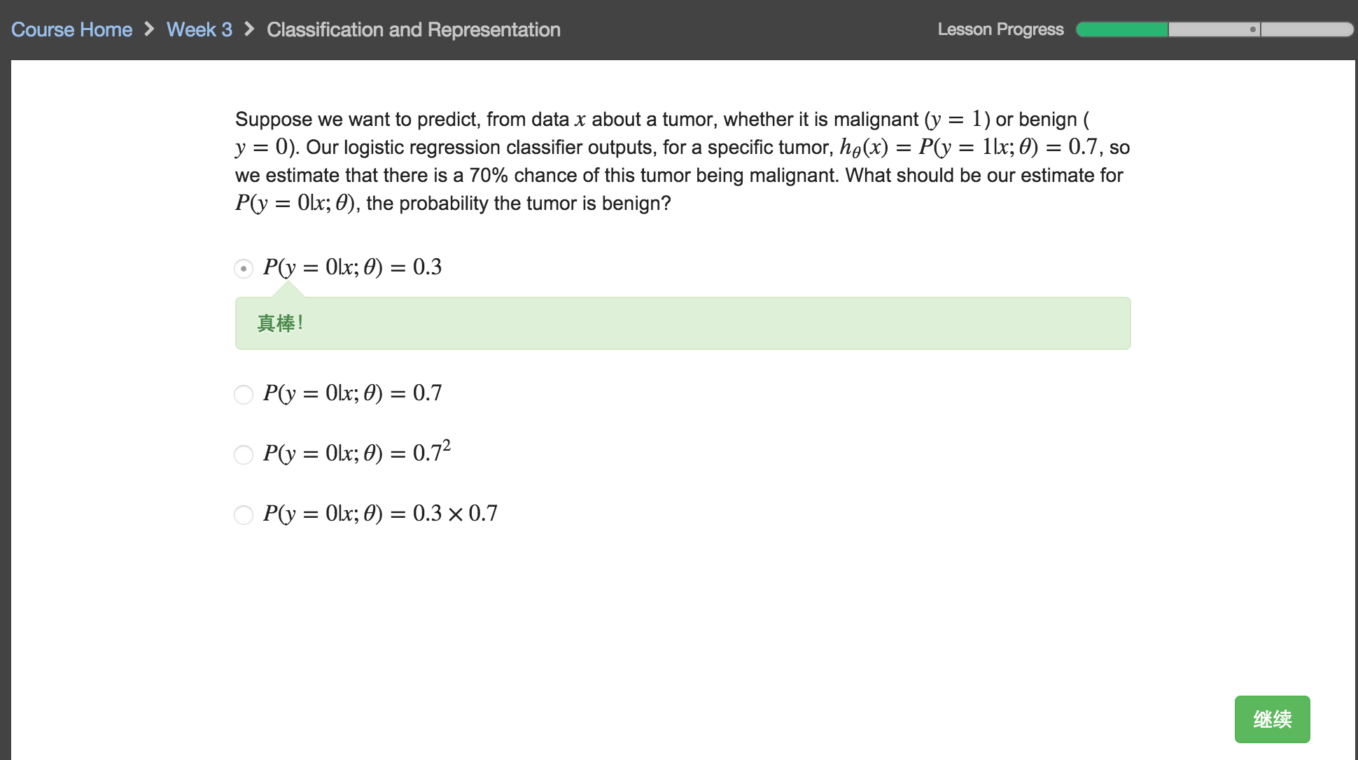
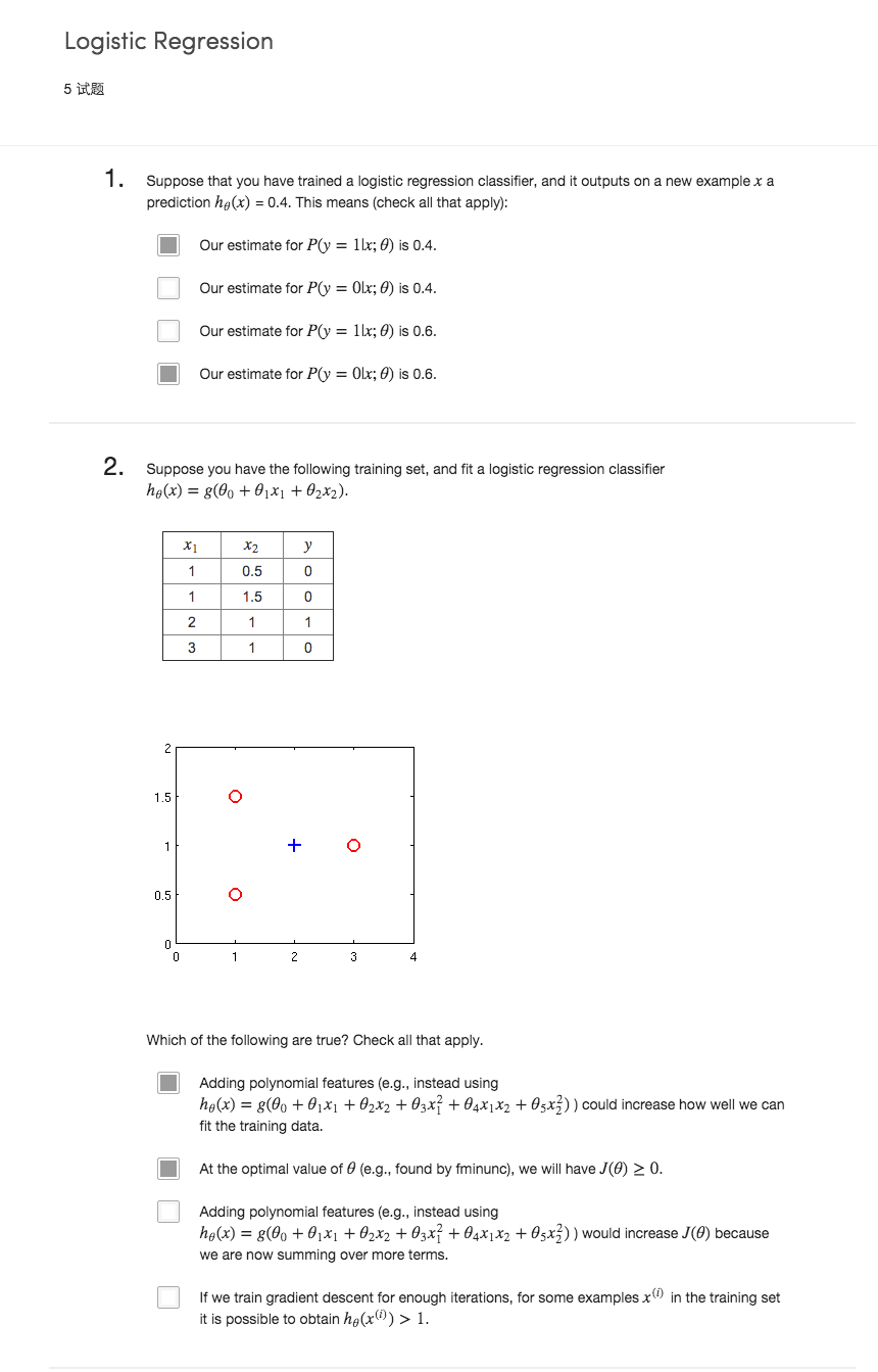
hθ(x)的作用是,对于给定的输入变量,根据选择的参数计算输出变量=1 的可能性(estimated probablity)即

$$h_\theta(x) = P(y=1 | x ; \theta)= 1 - P(y=0 | x ; \theta)$$

例如,如果对于给定的 x,通过已经确定的参数计算得出 hθ(x)=0.7,则表示有百分之70 的几率 y 为正向类,相应地 y 为负向类的几率为 1-0.7=0.3。

Our hypothesis should satisfy:
$\large y \in \lbrace 0,1 \rbrace$
Our new form uses the “Sigmoid Function,” also called the “Logistic Function”:
$\large \begin{align*} & h_\theta (x) = g ( \theta^T x ) \newline \newline & z = \theta^T x \newline & g(z) = \dfrac{1}{1 + e^{-z}} \end{align*}$

The function g(z), shown here, maps any real number to the (0, 1) interval, making it useful for transforming an arbitrary-valued function into a function better suited for classification.
We start with our old hypothesis (linear regression), except that we want to restrict the range to 0 and 1. This is accomplished by plugging θTx into the Logistic Function.
hθ will give us the probability that our output is 1. For example, hθ(x)=0.7 gives us the probability of 70% that our output is 1.

$\large \begin{align*} & h_\theta(x) = P(y=1 | x ; \theta) = 1 - P(y=0 | x ; \theta) \newline & P(y = 0 | x;\theta) + P(y = 1 | x ; \theta) = 1 \end{align*}$

Our probability that our prediction is 0 is just the opposite of our probability that it is 1 (e.g. if probability that it is 1 is 70%, then the probability that it is 0 is 30%).

---

3 判定边界 Decision Boundary

在逻辑回归中,我们预测:

• 当 hθ大于等于 0.5 时,预测 y=1
• 当 hθ小于 0.5 时,预测 y=0

根据上面绘制出的 S形函数图像,我们知道当

• z=0 时 g(z)=0.5
• z>0 时 g(z)>0.5
• z<0 时 g(z)<0.5

又$z = \theta^T x$,即:

$$\begin{align*} & \theta^T x \geq 0 \rightarrow y = 1 \newline & \theta^T x < 0 \rightarrow y = 0 \newline \end{align*}$$
现在假设我们有一个模型:  并且参数θ是向量[-3 1 1]。 则当-3+x1+x2 大于等于 0,即 x1+x2 大于等于 3 时,模型将预测 y=1。

我们可以绘制直线 x1+x2=3,这条线便是我们模型的分界线,将预测为 1 的区域和预测为 0 的区域分隔开。

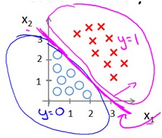
假使我们的数据呈现这样的分布情况,怎样的模型才能适合呢?

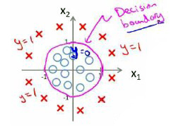
因为需要用曲线才能分隔 y=0 的区域和 y=1 的区域,我们需要二次方特征:



假设参数是[-1 0 0 1 1],则我们得到的判定边界恰好是圆点在原点且半径为 1 的圆形。 我们可以用非常复杂的模型来适应非常复杂形状的判定边界。

In order to get our discrete 0 or 1 classification, we can translate the output of the hypothesis function as follows:

$$\begin{align*} & h_\theta(x) \geq 0.5 \rightarrow y = 1 \newline & h_\theta(x) < 0.5 \rightarrow y = 0 \newline \end{align*}$$
The way our logistic function g behaves is that when its input is greater than or equal to zero, its output is greater than or equal to 0.5:
$$\begin{align*} & g(z) \geq 0.5 \newline & when \; z \geq 0 \end{align*}$$

Remember.-

$$\begin{align*} z=0, e^{0}=1, g(z)=1/2\newline z \to \infty, e^{-\infty} \to 0, g(z)=1 \newline z \to -\infty, e^{\infty}\to \infty, g(z)=0 \end{align*}$$

So if our input to g is $\theta^T X$, then that means:

$$\begin{align*} & h_\theta(x) = g(\theta^T x) \geq 0.5 \newline & when \; \theta^T x \geq 0 \end{align*}$$

From these statements we can now say:

$$\begin{align*} & \theta^T x \geq 0 \rightarrow y = 1 \newline & \theta^T x < 0 \rightarrow y = 0 \newline \end{align*}$$

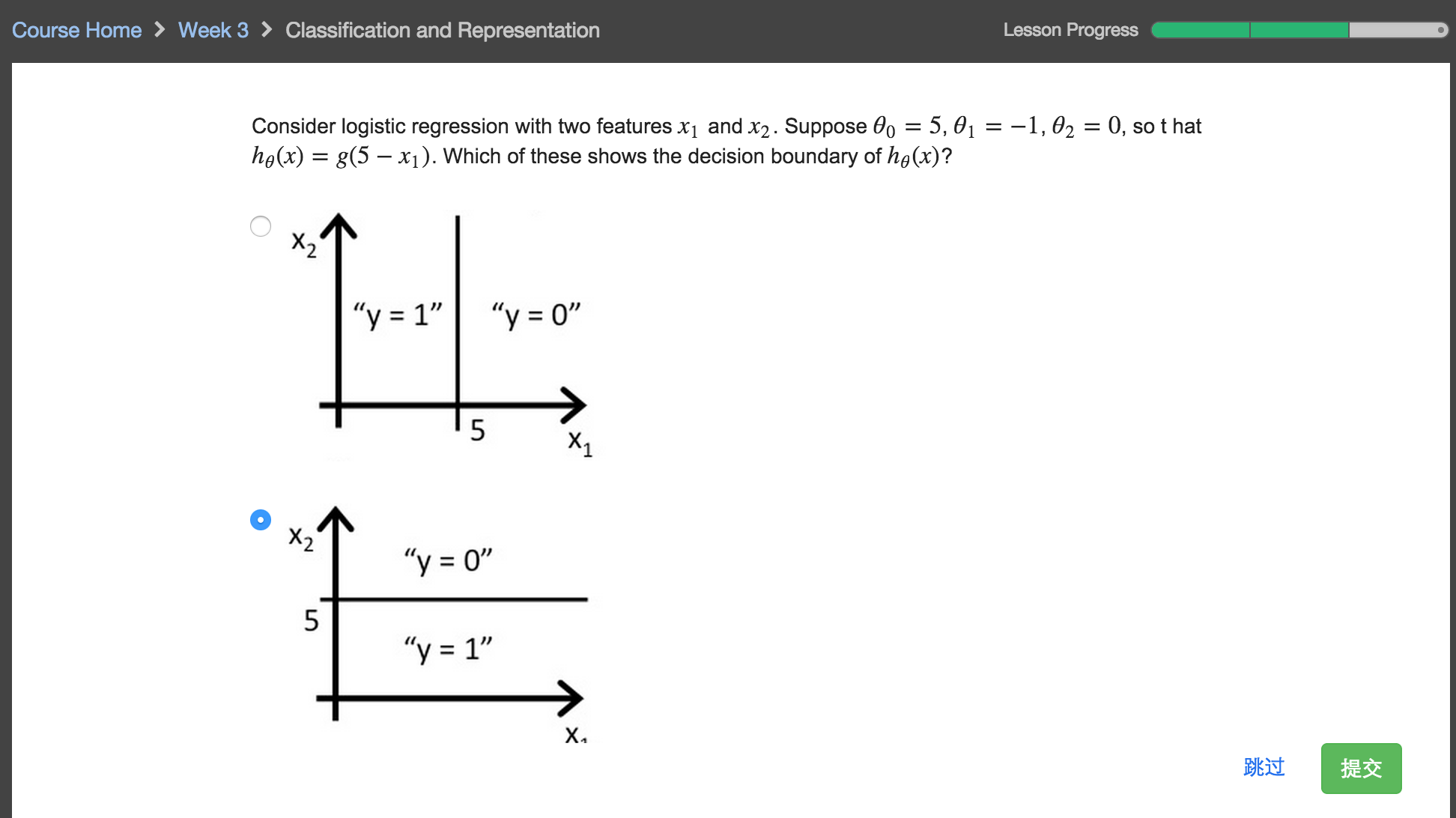
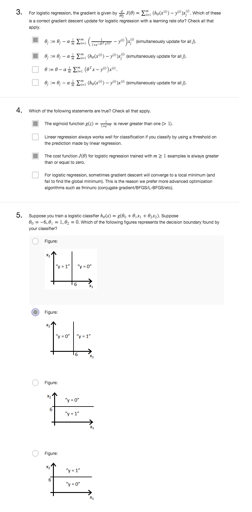
The decision boundary is the line that separates the area where y=0 and where y=1. It is created by our hypothesis function.
Example:

$$\begin{align*} & \theta = \begin{bmatrix}5 \newline -1 \newline 0\end{bmatrix} \newline & y = 1 \; if \; 5 + (-1) x_1 + 0 x_2 \geq 0 \newline & 5 - x_1 \geq 0 \newline & - x_1 \geq -5 \newline & x_1 \leq 5 \newline \end{align*}$$
Our decision boundary then is a straight vertical line placed on the graph where x1=5, and everything to the left of that denotes y=1, while everything to the right denotes y=0.
Again, the input to the sigmoid function g(z) (e.g. $\theta^T X$) need not be linear, and could be a function that describes a circle (e.g. $z = \theta_0 + \theta_1 x_1^2 +\theta_2 x_2^2$) or any shape to fit our data.

---

4 代价函数 Cost Function

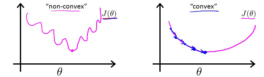
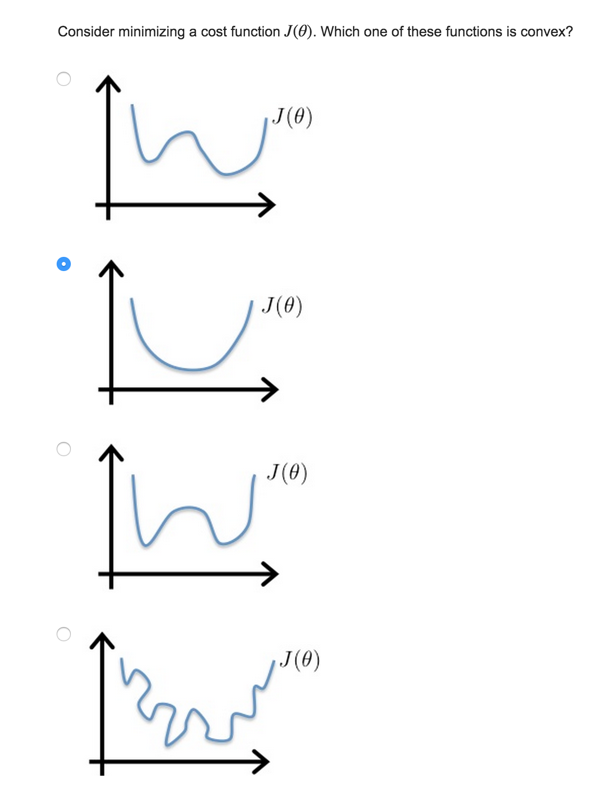
对于线性回归模型,我们定义的代价函数是所有模型误差的平方和。理论上来说,我们也可以对逻辑回归模型沿用这个定义,但是问题在于,当我们将 $h_\theta (x) = \dfrac{1}{1 + e^{-z}}$带入到这样定义了的代价函数中时,我们得到的代价函数将是一个非凸函数(non-convex function)。
这意味着我们的代价函数有许多局部最小值,这将影响梯度下降算法寻找全局最小值。

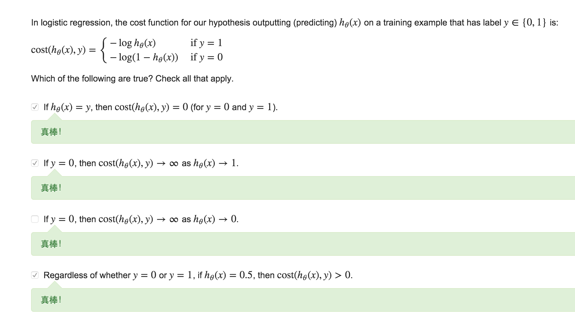
因此我们重新定义逻辑回归的代价函数为:

$$\begin{align*} & J(\theta) = \dfrac{1}{m} \sum_{i=1}^m \mathrm{Cost}(h_\theta(x^{(i)}),y^{(i)}) \newline & \mathrm{Cost}(h_\theta(x),y) = -\log(h_\theta(x)) \; & \text{if y = 1} \newline & \mathrm{Cost}(h_\theta(x),y) = -\log(1-h_\theta(x)) \; & \text{if y = 0} \end{align*}$$
hθ(x)与 Cost(hθ(x),y)之间的关系如下图所示:

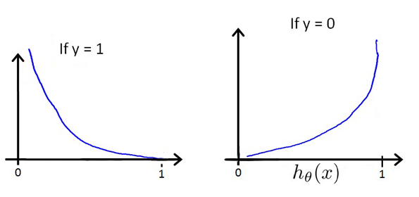
这样构建的 Cost(hθ(x),y)函数的特点是:当实际的 y=1 且 hθ也为 1 时误差为 0,当 y=1 但 h θ不为 1 时误差随着 hθ的变小而变大;当实际的 y=0 且 hθ也为 0 时代价为 0,当 y=0 但 hθ 不为 0 时误差随着 hθ的变大而变大。

We cannot use the same cost function that we use for linear regression because the Logistic Function will cause the output to be wavy, causing many local optima. In other words, it will not be a convex function.
Instead, our cost function for logistic regression looks like:

$$\begin{align*} & J(\theta) = \dfrac{1}{m} \sum_{i=1}^m \mathrm{Cost}(h_\theta(x^{(i)}),y^{(i)}) \newline & \mathrm{Cost}(h_\theta(x),y) = -\log(h_\theta(x)) \; & \text{if y = 1} \newline & \mathrm{Cost}(h_\theta(x),y) = -\log(1-h_\theta(x)) \; & \text{if y = 0} \end{align*}$$

The more our hypothesis is off from y, the larger the cost function output. If our hypothesis is equal to y, then our cost is 0:

$$\begin{align*} & \mathrm{Cost}(h_\theta(x),y) = 0 \text{ if } h_\theta(x) = y \newline & \mathrm{Cost}(h_\theta(x),y) \rightarrow \infty \text{ if } y = 0 \; \mathrm{and} \; h_\theta(x) \rightarrow 1 \newline & \mathrm{Cost}(h_\theta(x),y) \rightarrow \infty \text{ if } y = 1 \; \mathrm{and} \; h_\theta(x) \rightarrow 0 \newline \end{align*}$$

If our correct answer ‘y’ is 0, then the cost function will be 0 if our hypothesis function also outputs 0. If our hypothesis approaches 1, then the cost function will approach infinity.
If our correct answer ‘y’ is 1, then the cost function will be 0 if our hypothesis function outputs 1. If our hypothesis approaches 0, then the cost function will approach infinity.
Note that writing the cost function in this way guarantees that $J(\theta)$ is convex for logistic regression.

---

5 Simplified Cost Function and Gradient Descent

将构建的 Cost(hθ(x),y)简化如下:

We can compress our cost function’s two conditional cases into one case:

$$\mathrm{Cost}(h_\theta(x),y) = - y \; \log(h_\theta(x)) - (1 - y) \log(1 - h_\theta(x))$$
Notice that when y is equal to 1, then the second term ((1−y)log(1−hθ(x))) will be zero and will not affect the result. If y is equal to 0, then the first term (−ylog(hθ(x))) will be zero and will not affect the result.
We can fully write out our entire cost function as follows:
带入代价函数得到:
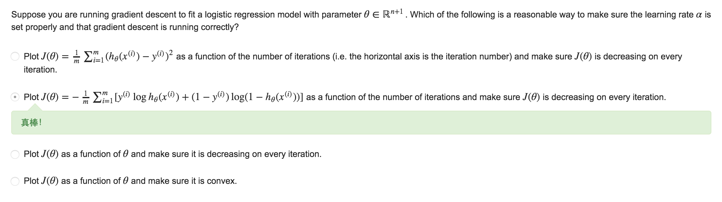
$\large J(\theta) = - \frac{1}{m} \displaystyle \sum_{i=1}^m [y^{(i)}\log (h_\theta (x^{(i)})) + (1 - y^{(i)})\log (1 - h_\theta(x^{(i)}))]$

A vectorized implementation is:
$\large J\left(\theta\right) = -\frac{1}{m}\left(\log\left(g\left(X\theta\right)\right)^{T}y+\log\left(1-g\left(X\theta\right)\right)^{T}\left(1-y\right)\right)$

---

5.1 Gradient Descent

一般的梯度下降算法：
Remember that the general form of gradient descent is:

$$\begin{align*} & Repeat \; \lbrace \newline & \; \theta_j := \theta_j - \alpha \dfrac{\partial}{\partial \theta_j}J(\theta) \newline & \rbrace \end{align*}$$

在得到这样一个代价函数以后,我们便可以用梯度下降算法来求得能使代价函数最小的参数了。 算法为:
We can work out the derivative part using calculus to get:

$$\begin{align*} & Repeat \; \lbrace \newline & \; \theta_j := \theta_j - \frac{\alpha}{m} \sum_{i=1}^m (h_\theta(x^{(i)}) - y^{(i)}) x_j^{(i)} \newline & \rbrace \end{align*}$$

注:虽然得到的梯度下降算法表面上看上去与线性回归的梯度下降算法一样,但是这里的 hθ (x)=g(θTX)与线性回归中不同,所以实际上是不一样的。另外,在运行梯度下降算法之前,进行特征缩放依旧是非常必要的。
Notice that this algorithm is identical to the one we used in linear regression. We still have to simultaneously update all values in theta.
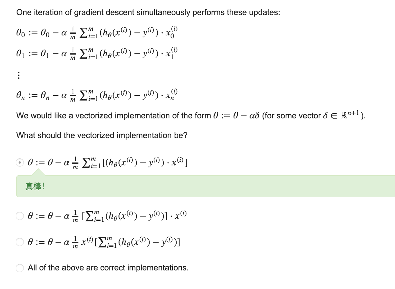
向量化的实现：
A vectorized implementation is:

$\large \theta := \theta - \frac{\alpha}{m} X^{T} (g(X \theta ) - \vec{y})$

---

---

5.2 J(θ)的偏导数 Partial derivative of J(θ)

首先计算S函数的偏导数：
First calculate derivative of sigmoid function (it will be useful while finding partial derivative of $J(\theta)$:

$$\begin{equation} \sigma(x)' =\left(\frac{1}{1+e^{-x}}\right)' =\frac{-(1+e^{-x})'}{(1+e^{-x})^2} =\frac{-1'-(e^{-x})'}{(1+e^{-x})^2} =\frac{0-(-x)'(e^{-x})}{(1+e^{-x})^2} =\frac{-(-1)(e^{-x})}{(1+e^{-x})^2} =\frac{e^{-x}}{(1+e^{-x})^2} =\left(\frac{1}{1+e^{-x}}\right)\left(\frac{e^{-x}}{1+e^{-x}}\right) =\sigma(x)\left(\frac{+1-1 + e^{-x}}{1+e^{-x}}\right) =\sigma(x)\left(\frac{1 + e^{-x}}{1+e^{-x}} - \frac{1}{1+e^{-x}}\right) =\sigma(x)(1 - \sigma(x)) \end{equation}$$
计算J(θ)的偏导数：
Now we are ready to find out resulting partial derivative:

$$\begin{align*} \frac{\partial}{\partial \theta_j} J(\theta) &= \frac{\partial}{\partial \theta_j} \frac{-1}{m}\sum_{i=1}^m \left [ y^{(i)} log (h_\theta(x^{(i)})) + (1-y^{(i)}) log (1 - h_\theta(x^{(i)})) \right ] \newline &= - \frac{1}{m}\sum_{i=1}^m \left [ y^{(i)} \frac{\partial}{\partial \theta_j} log (h_\theta(x^{(i)})) + (1-y^{(i)}) \frac{\partial}{\partial \theta_j} log (1 - h_\theta(x^{(i)})) \right ] \newline &= - \frac{1}{m}\sum_{i=1}^m \left [ \frac{y^{(i)} \frac{\partial}{\partial \theta_j} h_\theta(x^{(i)})}{h_\theta(x^{(i)})} + \frac{(1-y^{(i)})\frac{\partial}{\partial \theta_j} (1 - h_\theta(x^{(i)}))}{1 - h_\theta(x^{(i)})} \right ] \newline &= - \frac{1}{m}\sum_{i=1}^m \left [ \frac{y^{(i)} \frac{\partial}{\partial \theta_j} \sigma(\theta^T x^{(i)})}{h_\theta(x^{(i)})} + \frac{(1-y^{(i)})\frac{\partial}{\partial \theta_j} (1 - \sigma(\theta^T x^{(i)}))}{1 - h_\theta(x^{(i)})} \right ] \newline &= - \frac{1}{m}\sum_{i=1}^m \left [ \frac{y^{(i)} \sigma(\theta^T x^{(i)}) (1 - \sigma(\theta^T x^{(i)})) \frac{\partial}{\partial \theta_j} \theta^T x^{(i)}}{h_\theta(x^{(i)})} + \frac{- (1-y^{(i)}) \sigma(\theta^T x^{(i)}) (1 - \sigma(\theta^T x^{(i)})) \frac{\partial}{\partial \theta_j} \theta^T x^{(i)}}{1 - h_\theta(x^{(i)})} \right ] \newline &= - \frac{1}{m}\sum_{i=1}^m \left [ \frac{y^{(i)} h_\theta(x^{(i)}) (1 - h_\theta(x^{(i)})) \frac{\partial}{\partial \theta_j} \theta^T x^{(i)}}{h_\theta(x^{(i)})} - \frac{(1-y^{(i)}) h_\theta(x^{(i)}) (1 - h_\theta(x^{(i)})) \frac{\partial}{\partial \theta_j} \theta^T x^{(i)}}{1 - h_\theta(x^{(i)})} \right ] \newline &= - \frac{1}{m}\sum_{i=1}^m \left [ y^{(i)} (1 - h_\theta(x^{(i)})) x^{(i)}_j - (1-y^{(i)}) h_\theta(x^{(i)}) x^{(i)}_j \right ] \newline &= - \frac{1}{m}\sum_{i=1}^m \left [ y^{(i)} (1 - h_\theta(x^{(i)})) - (1-y^{(i)}) h_\theta(x^{(i)}) \right ] x^{(i)}_j \newline &= - \frac{1}{m}\sum_{i=1}^m \left [ y^{(i)} - y^{(i)} h_\theta(x^{(i)}) - h_\theta(x^{(i)}) + y^{(i)} h_\theta(x^{(i)}) \right ] x^{(i)}_j \newline &= - \frac{1}{m}\sum_{i=1}^m \left [ y^{(i)} - h_\theta(x^{(i)}) \right ] x^{(i)}_j \newline &= \frac{1}{m}\sum_{i=1}^m \left [ h_\theta(x^{(i)}) - y^{(i)} \right ] x^{(i)}_j \end{align*}$$

---

6 高级优化 Advanced Optimization

一些梯度下降算法之外的选择:
除了梯度下降算法以外还有一些常被用来令代价函数最小的算法,这些算法更加复杂和优越, 而且通常不需要人工选择学习率,通常比梯度下降算法要更加快速。这些算法有:

• 共轭梯度 (Conjugate Gradient)
• 局部优化法(Broyden fletcher goldfarb shann,BFGS)
• 有限内存局部优化法(LBFGS)

“Conjugate gradient”, “BFGS”, and “L-BFGS” are more sophisticated, faster ways to optimize theta instead of using gradient descent. A. Ng suggests you do not write these more sophisticated algorithms yourself (unless you are an expert in numerical computing) but use them pre-written from libraries. Octave provides them.
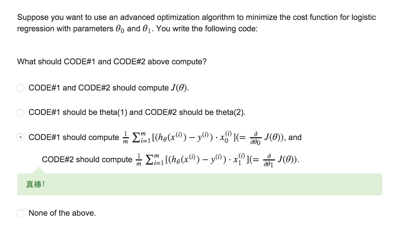
We first need to provide a function that computes the following two equations:
$\large \begin{align*} & J(\theta) \newline & \dfrac{\partial}{\partial \theta_j}J(\theta)\end{align*}$

We can write a single function that returns both of these:

function [jVal, gradient] = costFunction(theta)
  jval = [...code to compute J(theta)...];
  gradient = [...code to compute derivative of J(theta)...];
end

fminunc 是 matlab 和 octave 中都带的一个最小值优化函数,使用时我们需要提供代价函数 和每个参数的求导,下面是 octave 中使用 fminunc 函数的代码示例:

Then we can use octave’s “fminunc()” optimization algorithm along with the “optimset()” function that creates an object containing the options we want to send to “fminunc()”. (Note: the value for MaxIter should be an integer, not a character string - errata in the video at 7:30)

options = optimset('GradObj', 'on', 'MaxIter', 100);
initialTheta = zeros(2,1);
[optTheta, functionVal, exitFlag] = fminunc(@costFunction, initialTheta, options);

We give to the function “fminunc()” our cost function, our initial vector of theta values, and the “options” object that we created beforehand.
Note: If you use matlab, be aware that “fminunc()” is not available in the base installation - you also need to install the Optimization Toolbox http://www.mathworks.com/help/optim/ug/fminunc.html

---

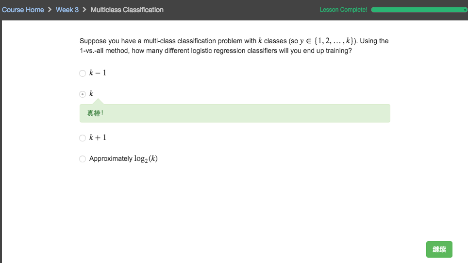
7 多分类 Multiclass Classification: One-vs-all

判断依据。例如我们要预测天气情况分四种类型:晴天、多云、下雨或下雪。



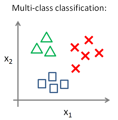
一种解决这类问题的途径是采用一对多(One-vs-All)方法。在一对多方法中,我们将多类分类问题转化成二元分类问题。为了能实现这样的转变,我们将多个类中的一个类标记为正向类(y=1),然后将其他所有类都标记为负向类,这个模型记作  $h_\theta^{(1)}(x)$ 。
接着,类似地第我们选择另一个类标记为正向类(y=2),再将其它类都标记为负向类,将这个模型记作$h_\theta^{(2)}(x)$  ,依此类推。
最后我们得到一系列的模型简记为:

$$h_\theta^{(i)}(x) = P(y = i | x ; \theta) i \in \lbrace0, 1 ... n\rbrace$$
Now we will approach the classification of data into more than two categories. Instead of y = {0,1} we will expand our definition so that y = {0,1…n}.
In this case we divide our problem into n+1 binary classification problems; in each one, we predict the probability that ‘y’ is a member of one of our classes.

$$\begin{align*} & y \in \lbrace0, 1 ... n\rbrace \newline & h_\theta^{(0)}(x) = P(y = 0 | x ; \theta) \newline & h_\theta^{(1)}(x) = P(y = 1 | x ; \theta) \newline & \cdots \newline & h_\theta^{(n)}(x) = P(y = n | x ; \theta) \newline & \mathrm{prediction} = \max_i( h_\theta ^{(i)}(x) )\newline \end{align*}$$



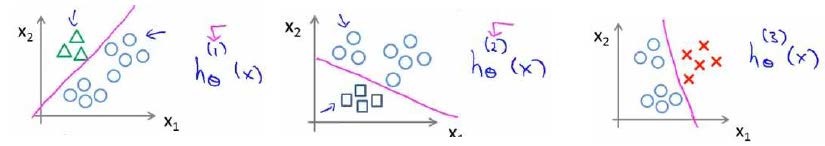
最后,在我们需要做预测时,我们将所有的分类机都运行一遍,然后对每一个输入变量,都选 择最高可能性的输出变量。
We are basically choosing one class and then lumping all the others into a single second class. We do this repeatedly, applying binary logistic regression to each case, and then use the hypothesis that returned the highest value as our prediction.

---