Multi-task Learning

最新推荐文章于 2022-12-29 21:18:33 发布

大眼呆萌君

最新推荐文章于 2022-12-29 21:18:33 发布

阅读量587

点赞数

分类专栏：专题

本文链接：https://blog.csdn.net/my_god2008/article/details/53414575

版权

专题专栏收录该内容

3 篇文章 0 订阅

订阅专栏

基于Supervised Learning Lecture 8

Multi-task learning
- Mathematical formulation
Linear MTL
- Regularisers for linear MTL
  - Quadratic regulariser
  - Structured sparsity
Clustered MTL
Further topics
- Transferring to new tasks
  - Case of the variance regulariser
  - Informal reasoning
Take home message

Multi-task learning

Multi-task learning (MTL) is an approach to machine learning that learns a problem together with other related problems at the same time, using a shared representation. 1
The goal of MTL is to improve the performance of learning algorithms by learning classifiers for multiple tasks jointly.
Typical scenario: many tasks many tasks but only few examples per task. If $n < d$ we don’t have enough data to learn the tasks one by one. However, if the tasks are related and set $\cal S$ or the associated regularizer captures such relationships in a simple way, learning the tasks jointly greatly improves over independent task learning (ITL).
When problems (tasks) are closely related, learning in parallel can be more efficient than learning tasks independently. Also, this often leads to a better model for the main task, because it allows the learner to use the commonality among the tasks.
Applications: Learning a set of linear classi ers for related objects
(cars, lorries, bicycles), user modelling, multiple object detection in scenes, affective computing, bioinformatics, health informatics, marketing science, neuroimaging, NLP, speech…
Further categorisation is possible, e.g. hierarchical models, clustering of tasks.
The ideas can be extended to non-linear cases through RKHS.

Mathematical formulation

Fix probability measures $\mu_1, \cdots, \mu_T$ on $\mathbb{R}^d \times \mathbb{R}$
– T tasks
– Each task is a probability measure, e.g. $\mu_t(x,y)=P(x)\delta(\left\langle w^*,x\right\rangle-y)$ . $\delta$ is a deterministic function, interpreted as the conditional probability and $w^x$ is an underlying parameter
– $\mathbb{R}^d$ can also be a Hilbert space
Draw data: $(x_{t1 \> \textit{vector}},y_{t1 \> \textit{scalar}}), \cdots,(x_{tn},y_{tn}) \sim \mu_t, \quad t=1, \cdots, T$ (in practice n may vary with t)
Learning method:

$min (f 1, \dots, f T) \in F 1 T \sum t = 1 T 1 n \sum i = 1 n ℓ (y t i, f t (x t i))$ $\min_{(f_1,\cdots,f_T) \in \cal F} \frac{1}{T} \sum_{t=1}^T \frac{1}{n} \sum_{i=1}^n \ell(y_{ti},f_t(x_{ti}))$

where $\cal F$ is a set of vector-value functions. A standard choice is a ball in a RKHS, which models interactions between the tasks in the sense that functions with small norm have strongly related components.
Goal is to minimise the multi-task error

$R (f 1, \dots, f T) = 1 T \sum t = 1 T E (x, y) \sim μ t ℓ (y t i, f t (x t i))$ $R(f_1,\cdots,f_T)=\frac{1}{T} \sum_{t=1}^T \underset{(x,y) \sim \mu_t}{\mathbb{E}} \ell(y_{ti},f_t(x_{ti}))$

Linear MTL

“task” = “linear model”
– Regression: $y_{ti}=\left\langle w_t^*, x_{ti} \right\rangle + \epsilon_{ti}$
– Binary classification: $y_{ti}=sign(\left\langle w_t^*, x_{ti} \right\rangle) \epsilon_{ti}$
Learning method: $\min_{(w_1,\cdots,w_T) \in \cal S} \frac{1}{T} \sum_{t=1}^T \frac{1}{n} \sum_{i=1}^n \ell(y_{ti},\left\langle w_t^*, x_{ti} \right\rangle)$ . Here, $\cal S$ incorporates the prior knowledge about the regression vector and encourages “common structure” among tasks, e.g. the ball of a matrix norm or other regulariser.
The multitask error of $W=[w_1, \cdots,w_T]$ is: $R(W)=\frac{1}{T} \sum_{t=1}^T \underset{(x,y) \sim \mu_t}{\mathbb{E}} \ell(y_{ti},\left\langle w_t,x \right\rangle)$
It is possible to give bounds on the uniform deviation
$sup W \in S {R (W) - 1 T \sum t = 1 T 1 n \sum i = 1 n ℓ (y t i, ⟨ w t, x t i ⟩)}$ $\sup_{W \in \cal S} \{ R(W)-\frac{1}{T} \sum_{t=1}^T \frac{1}{n} \sum_{i=1}^n \ell(y_{ti},\left\langle w_t, x_{ti} \right\rangle) \}$
and derive bounds for excess error
$R (W^) - min W \in S R (W)$ $R(\hat W)-\min_{W \in \cal S}R(W)$

Regularisers for linear MTL

Often we drop the constraint (i.e. $W \in \cal S$ ) and consider the penalty methods

min w 1, \dots, w T 1 T \sum t = 1 T 1 n \sum i = 1 n ℓ (y t i, ⟨ w t, x t i ⟩) + λ Ω (w 1, \dots, w T)

$\min_{w_1,\cdots,w_T}\frac{1}{T} \sum_{t=1}^T \frac{1}{n} \sum_{i=1}^n \ell(y_{ti},\left\langle w_t, x_{ti} \right\rangle)+\lambda\Omega(w_1,\cdots,w_T)$
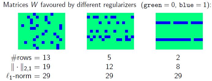
Different regularisers encourage different types of commonalities between the tasks:

variance (or other convex quadratic regularisers) encourage closeness to mean
$Ω var = 1 T \sum t = 1 T | | w t | | 2 + 1 - γ γ V a r (w 1, \dots, w T)$ $\Omega_\text{var}=\frac{1}{T}\sum_{t=1}^{T}\left|\left| w_t \right| \right|^2+\frac{1-\gamma}{\gamma}Var(w_1,\cdots,w_T)$
Joint sparsity (or other structured sparsity regularisers) encourage few shared variables
$| | W | | 2, 1 : = \sum j = 1 d \sum t = 1 T w 2 t j - - - - - -  ⎷  $ $\left|\left|W\right|\right|_{2,1}:=\sum_{j=1}^d\sqrt{\sum_{t=1}^Tw_{tj}^2}$
Trace norm (or other spectral regularisers which promote low rank solutions) encourage few shared features
$| | w 1, \dots, w T | | t r$ $\left|\left|w_1,\cdots,w_T\right|\right|_{tr}$
– extension of joint sparsity; rotate the initial data representation
– The $l_1$ norm of SVD of this matrix is bounded, so favour low-rank representation (i.e. common low-dimensional subspace)
More sophisticated regularisers which combine the above, promote clustering of tasks, etc.

Quadratic regulariser

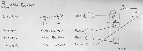
general quadratic regulariser
$Ω var = \sum s, t = 1 T ⟨ w s, E s t w t ⟩$ $\Omega_\text{var}=\sum_{s,t=1}^{T} \left\langle w_s,E_{st}w_t \right\rangle$
where the matrix $E=(E_{st})_{s,t=1}^{T} \in \mathbb{R}^{dT \times dT}$ is positive definite.
variance regulariser
Let $\gamma \in [0,1]$ and
$Ω var = 1 T \sum t = 1 T | | w t | | 2 + 1 - γ γ V a r (w 1, \dots, w T) = 1 T \sum t = 1 T | | w t | | 2 + 1 - γ γ \sum t = 1 T | | w t - w ¯ | | 22$ $\begin{align} \Omega_\text{var} &=\frac{1}{T}\sum_{t=1}^{T}\left|\left| w_t \right| \right|^2+\frac{1-\gamma}{\gamma}Var(w_1,\cdots,w_T)\\ &=\frac{1}{T}\sum_{t=1}^{T}\left|\left| w_t \right| \right|^2+\frac{1-\gamma}{\gamma} \sum_{t=1}^{T} \left|\left| w_t - \bar w \right|\right|^2_2 \end{align}$
– $\gamma=1$ : independent tasks; $\gamma=0$ : identical tasks
– regulariser favours weight vectors which are close to its mean.
– If we are working on SVM with hinge loss, the objective function is a compromise between maximising individual margins and minimising the variance (i.e. keeping the tasks close to each other)
Link to the kernel methods (quadratic regulariser)
The problem
$min w 1, \dots, w T 1 T \sum t = 1 T 1 n \sum i = 1 n ℓ (y t i, ⟨ w t, x t i ⟩) + λ \sum s, t = 1 T ⟨ w s, E s t w t ⟩$ $\min_{w_1,\cdots,w_T}\frac{1}{T} \sum_{t=1}^T \frac{1}{n} \sum_{i=1}^n \ell(y_{ti},\left\langle w_t, x_{ti} \right\rangle)+\lambda\sum_{s,t=1}^{T} \left\langle w_s,E_{st}w_t \right\rangle$
is equivalent to

$min v 1 T \sum t = 1 T 1 n \sum i = 1 n ℓ (y t i, ⟨ v, B t x t i ⟩) + λ ⟨ v, v ⟩ (1)$ $\min_v\frac{1}{T} \sum_{t=1}^T \frac{1}{n} \sum_{i=1}^n \ell(y_{ti},\left\langle v, B_t x_{ti} \right\rangle)+\lambda \left\langle v,v \right\rangle \tag{1}$

where $B_t$ are $p \times d$ matrices (typically $p \gg d$ ) linked to $E$ by $E=(B^TB)^{-1}, B_{\textit{dim=p×dT}}=[B_1, \cdots, B_T]_{\textit{concatenate by columns}}$ and $w_t=(B_t)^T v_t$
Interpretation:
– We learn a single function $(x,t) \mapsto f_t(x)$ using the feature map $(x,t) \mapsto B_t(x)$ and corresponding multitask kernel $K((x_1,t_1),(x_2,t_2))=\left\langle B_{t1}x_1, B_{t2}x_2 \right\rangle$
– Writing $\left\langle v,B_tx\right\rangle = \left\langle B_t^Tv,x\right\rangle$ , we interpret this as having a single regression vector which is transformed by matrix $B_t$ to obtain the task specific weight vector.
Link to the kernel methods (variance regulariser)
The problem
$min w 1, \dots, w T 1 T n \sum t, i ℓ (y t i, ⟨ w t, x t i ⟩) + λ (1 T \sum t = 1 T | | w t | | 2 + 1 - γ γ V a r (w 1, \dots, w T))$ $\min_{w_1,\cdots,w_T}\frac{1}{Tn} \sum_{t,i} \ell(y_{ti},\left\langle w_t, x_{ti} \right\rangle)+\lambda(\frac{1}{T}\sum_{t=1}^{T}\left|\left| w_t \right| \right|^2+\frac{1-\gamma}{\gamma}Var(w_1,\cdots,w_T))$
is equivalent to
$min w 0, u 1, \dots, u T 1 T n \sum t, i ℓ (y t i, ⟨ w 0 + u t, x t i ⟩) + λ (1 γ T \sum t = 1 T | | u t | | 2 + 1 1 - γ | | w 0 | | 2) (2)$ $\min_{w_0,u_1,\cdots,u_T}\frac{1}{Tn} \sum_{t,i} \ell(y_{ti},\left\langle w_0+u_t,x_{ti} \right\rangle)+\lambda (\frac{1}{\gamma T} \sum_{t=1}^T \left|\left| u_t \right|\right|^2+\frac{1}{1-\gamma} \left|\left| w_0 \right|\right|^2 ) \tag{2}$
by setting $w_t=w_0+u_t$ and minimise over $w_0$ .
It is of the form (1) with
$v B T t d i m = (T + 1) d \times d = ((1 - γ) - 1 2 w 0, (γ T) - 1 2 u 1, \dots, (γ T) - 1 2 u T) = [1 - γ - - - - \sqrt I d \times d, 0 d \times d, \dots, 0 d \times d                t-1, γ T - - - \sqrt I d \times d, 0 d \times d, \dots, 0 d \times d                T-t]$ $\begin{align} v&=((1-\gamma)^{-\frac{1}{2}}w_0,(\gamma T)^{-\frac{1}{2}}u_1, \cdots, (\gamma T)^{-\frac{1}{2}}u_T) \\ B_{t \> \textit{dim=(T+1)d×d}}^T&=[\sqrt{1-\gamma}\mathbf{I}_{d \times d}, \underbrace{\mathbf{0}_{d \times d}, \cdots, \mathbf{0}_{d \times d}}_\text{t-1}, \sqrt{\gamma T}\mathbf{I}_{d \times d}, \underbrace{\mathbf{0}_{d \times d}, \cdots, \mathbf{0}_{d \times d}}_\text{T-t}] \end{align}$
and the corresponding kernel $K((x_1,t_1),(x_2,t_2))=(1-\gamma + \gamma T \delta_{t_1t_2})\left\langle x_1,x_2 \right\rangle$
By writing (2) as the following, it is more apparent that we regularise around some common vector $w_0$
$min w 0 1 T \sum t = 1 T min w {1 n \sum i = 1 n ℓ (y t i, ⟨ w, x t i ⟩) + λ γ | | w - w 0 | | 2} + λ 1 - γ | | w 0 | | 2$ $\min_{w_0}\frac{1}{T} \sum_{t=1}^{T} \min_{w} \{\frac{1}{n}\sum_{i=1}^{n} \ell(y_{ti},\left\langle w,x_{ti} \right\rangle )+ \frac{\lambda}{\gamma} \left|\left| w-w_0 \right|\right|^2 \} +\frac{\lambda}{1-\gamma} \left|\left| w_0 \right|\right|^2$
More multitask kernels

Structured sparsity

general sparsity regulariser
$| | W | | 2, 1 : = \sum j = 1 d \sum t = 1 T w 2 t j - - - - - -  ⎷  $ $\left|\left|W\right|\right|_{2,1}:=\sum_{j=1}^d\sqrt{\sum_{t=1}^Tw_{tj}^2}$
– sum of the $l_2$ norm of the row of matrix
– encourages a matrix has only a few non-zero rows
– regression vectors are sparse, but the sparsity pattern is contained in a small cardinality

Clustered MTL

Further topics

Transferring to new tasks

Having found a feature map $h$ , to test it on the environment we
1) draw a task $\mu \sim \cal E$
2) draw a sample $\mathbf{z} \sim \mu^n$
3) run the algorithm to obtain $a \> (h)_\mathbf{z}={\hat f}_{h,\mathbf{z}} \circ h$
4) measure the loss of $a \> (h)_\mathbf{z}$ on a random pair $(x,y) \sim \mu$
The error associated with the algorithm $a \> (h)$ is
$R n (h) = E μ \sim E E z \sim μ n E (x, y) \sim μ [ℓ (a (h) z (x), y)]$ $R_n(h)=\mathbb{E}_{\mu \sim \cal E} \mathbb{E}_{\mathbf{z} \sim \mu^n} \mathbb{E}_{(x,y) \sim \mu} [\ell(a \>(h)_z(x),y)]$
The best value for a representation $h$ given complete knowledge of the environment is then
$min h \in H R n (h)$ $\min_{h \in \cal H}R_n(h)$
Compare to the very best we can do:

$R * = min h \in H E μ \sim E [min f \in F E (x, y) \sim μ ℓ (f (h (x)), y)]$ $R_*=\min_{h \in \cal H}\mathbb{E}_{\mu \sim \cal E} [\min_{f \in \cal F} \mathbb{E}_{(x,y) \sim \mu} \ell(f(h(x)),y)]$
The excess error associated with $h$ is then $R_n(h)-R_*$

Case of the variance regulariser

Training
$min w 0 1 T \sum t = 1 T min w {1 n \sum i = 1 n ℓ (y t i, ⟨ w, x t i ⟩ + λ γ | | w - w 0 | | 2} + λ 1 - γ | | w 0 | | 2$ $\min_{w_0}\frac{1}{T} \sum_{t=1}^{T} \min_{w} \{\frac{1}{n}\sum_{i=1}^{n} \ell(y_{ti},\left\langle w,x_{ti} \right\rangle+ \frac{\lambda}{\gamma} \left|\left| w-w_0 \right|\right|^2 \} +\frac{\lambda}{1-\gamma} \left|\left| w_0 \right|\right|^2$
Testing
$min w 1 n \sum i = 1 n ℓ (y i, ⟨ w, x i ⟩) + λ γ | | w - w 0 | | 2$ $\min_{w} \frac{1}{n}\sum_{i=1}^{n} \ell(y_{i},\left\langle w,x_{i} \right\rangle )+ \frac{\lambda}{\gamma} \left|\left| w-w_0 \right|\right|^2$
Error
$R n (w 0) = E μ \sim E E z \sim μ n E (x, y) \sim μ ℓ (y, ⟨ w 0 + w z, x) ⟩$ $R_n(w_0)=\mathbb{E}_{\mu \sim \cal E} \mathbb{E}_{\mathbf{z} \sim \mu^n} \mathbb{E}_{(x,y) \sim \mu} \ell (y,\left\langle {w_0+w_\mathbf{z},x}) \right\rangle$
Best we can do
$R * = min w 0 E μ \sim E [min w E (x, y) \sim μ ℓ (y, ⟨ w 0 + w, x) ⟩]$ $R_*=\min_{w_0}\mathbb{E}_{\mu \sim \cal E} [\min_{w} \mathbb{E}_{(x,y) \sim \mu} \ell (y,\left\langle {w_0+w,x}) \right\rangle]$
Excess error of $w_0$ : $R_n(w_0)-R_*$

Informal reasoning

The feature map $B$ learned from the training tasks can be used to learn a new task more quickly (a kind of bias learning heuristic).

Learn a new task by the method

minv{1n∑i=1nℓ(yt,⟨v,B∗xi⟩)+λ2||v||22}
- Give more weight to important features. In particular, if some eigenvalues of $G=B^*B$ are zero, the corresponding eigenvectors are discarded when learning a new task.
- In the case of diagonal matrices, some elements may be zero which results in a decreased number of parameters to learn.
- A statistical justification of an approach similar to this based on dictionary learning can be given.
- Take home message
  - MLT objective function
  - regulariser
  - link to kernel trick
  1. Multi-task learning, wikipedia
    https://en.wikipedia.org/wiki/Multi-task_learning ↩

大眼呆萌君

关注

0
点赞
踩
0

收藏

觉得还不错? 一键收藏
0
评论
Multi-task Learning

Multi-task learning and its definitionLinear MTLRegularisers for linear MTL (Quadratic regulariser, Structured sparsity)Clustered MTLFurther topics (Transferring to new tasks)
复制链接

扫一扫