吴恩达机器学习第三周学习笔记及编程作业答案

吴恩达机器学习第三周学习笔记及编程作业答案

一、理论基础
逻辑回归(Logistic Regression)
1. 分类问题
我们将因变量(dependent variable)可能属于的两个类分别称为负向类和正向类，其中 0 表示负向类，1 表示正向类


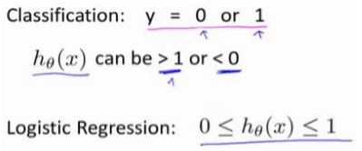
逻辑回归算法的性质是：它的输出值永远在 0 到 1 之间，逻辑回归算法实际上是一种分类算法。
2. 假说表示
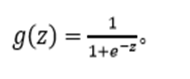
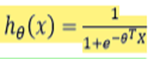
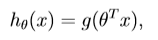
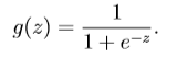
逻辑回归模型的假设是：其中：𝑋代表特征向量𝑔 代表逻辑函数（logistic function)是一个常用的逻辑函数为S形函数（Sigmoid function），公式为：

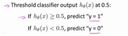
ℎ𝜃(𝑥)的作用是，对于给定的输入变量，根据选择的参数计算输出变量=1 的可能性，例如，如果对于给定的𝑥，通过已经确定的参数计算得出ℎ𝜃(𝑥) = 0.7，则表示有 70%的几率𝑦为正向类，相应地𝑦为负向类的几率为 1-0.7=0.3。
3. 判定边界
判定边界可以帮我们理解逻辑回归的假设函数在计算什么
例1：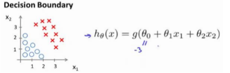
并且参数𝜃 是向量[-3 1 1]。 则当−3 + 𝑥1 + 𝑥2 ≥ 0，即𝑥1 + 𝑥2 ≥ 3时，模型将预测 𝑦 =1。 我们可以绘制直线𝑥1 + 𝑥2 = 3，这条线便是我们模型的分界线，将预测为 1 的区域和预测为 0 的区域分隔开。
例2：

因为需要用曲线才能分隔 𝑦 = 0 的区域和 𝑦 = 1 的区域，我们需要二次方特征：
是[-1 0 0 1 1]，则我们得到的判定边界恰好是圆点在原点且半径为 1 的圆形。
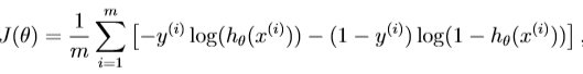
4. 代价函数
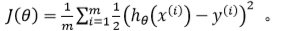
线性回归的代价函数为：

我们重新定义逻辑回归的代价函数为：

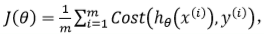
其中：

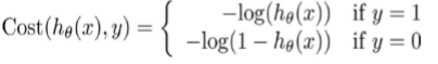
带入代价函数得到：

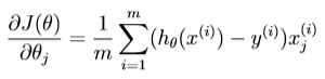
最小化代价函数的方法，是使用梯度下降法(gradient descent)。

线性回归假设函数：

逻辑函数假设函数：

注：即使更新参数的规则看起来基本相同，但由于假设的定义发生了变化，所以逻辑函数的梯度下降，跟线性回归的梯度下降实际上是两个完全不同的东西。
5. 高级优化
Fminunc函数
调用它的方式如下：
options=optimset(‘GradObj’,‘on’,‘MaxIter’,100);
initialTheta=zeros(2,1);
[optTheta, functionVal,
exitFlag]=fminunc(@costFunction, initialThet a, options);
解释：这个 options 变量作为一个数据结构可以存储你想要的 options，所以 GradObj 和 On，这里设置梯度目标参数为打开(on)，这意味着你现在确实要给这个算法提供一个梯度，然后设置最大迭代次数，比方说 100，我们给出一个𝜃 的猜测初始值，它是一个 2×1 的向量，那么这个命令就调用 fminunc，这个@符号表示指向我们刚刚定义的costFunction 函数的指针。如果你调用它，它就会使用众多高级优化算法中的一个，当然你也可以把它当成梯度下降，只不过它能自动选择学习速率𝛼，你不需要自己来做。然后它会尝试使用这些高级的优化算法，就像加强版的梯度下降法，为你找到最佳的𝜃值。
6. 正则化
6.1过拟合问题
正则化(regularization)可以改善或者减少过度拟合问题。

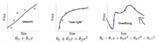
从左至右依次为：欠拟合、刚好、过拟合
过拟合问题解决办法：
1.丢弃一些不能帮助我们正确预测的特征。可以是手工选择保留哪些特征，或者使用一些模型选择的算法来帮忙（例如 PCA）
2.正则化。 保留所有的特征，但是减少参数的大小（magnitude）。
能防止过拟合问题的假设：

其中𝜆又称为正则化参数。
如果我们令 𝜆 的值很大的话，为了使 Cost Function 尽可能的小，所有的 𝜃 的值（不包括𝜃0）都会在一定程度上减小。但若 λ 的值太大了，那么𝜃（不包括𝜃0）都会趋近于 0，这样我们所得到的只能是一条平行于𝑥轴的直线。 所以对于正则化，我们要取一个合理的 𝜆 的值，这样才能更好的应用正则化。
6.2正则化线性回归、逻辑回归
正则化线性回归的代价函数为：

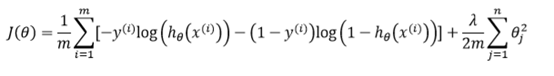
正则化的逻辑回归代价函数：

二、编程作业
1.plotData.m（Function to plot 2D classification data）：complete the code in plotData so that it displays a figure
like Figure 1, where the axes are the two exam scores, and the positive and negative examples are shown with different markers.

function plotData(X, y)  
%PLOTDATA Plots the data points X and y into a new figure   

%   PLOTDATA(x,y) plots the data points with + for the positive examples      
%   and o for the negative examples. X is assumed to be a Mx2 matrix.     
% Create New Figure  
 figure; hold on;  %holdon 函数的功能是将新的图像绘制在旧的之上
=load('ex2data1.txt');%下载ex2data1.txt中的数据  
X=data(:,[1,2]);%将data矩阵的1，2列赋值给X,因为在ex2data1.txt中第1，2列分别表示第一，二次的成绩  
y=data(:,3);%将data矩阵的第3列赋值给y，表示是否可以被录取  
=find(y==1);%当y=1的时候，是positive  
neg=find(y==0);  
plot(X(pos,1),X(pos,2),'k+','LineWidth',2,'MarkerSize',5);  
plot(X(neg,1),X(neg,2),'ko','MarkerFaceColor','r','MarkerSize',5);  
ld off;  
end 

2.sigmoid.m（Sigmoid Function） ：implement sigmoid function
logisticregression hypothesis：

sigmoid function：

function g = sigmoid(z)   
% You need to return the following variables correctly       
g = zeros(size(z));   
g(z)=1./(1+exp(-z));    
end  

解释：由于提示给出的是参数z，所以只需要实现sigmoid function即可
3.costFunction.m（Logistic Regression Cost Function）：implement the cost function and gradient for logistic regression
cost function in logistic regression：

function [J, grad] = costFunction(theta, X, y)  
m = length(y); % number of training examples     
% You need to return the following variables correctly        
J = 0;     
grad = zeros(size(theta));     
%法一  
J=(1/m)*(-y'*log(sigmoid(X*theta))-(1-y')*log(1-sigmoid(X*theta)));  
grad=(X'*((sigmoid(X*theta))-y))/m;  
%法二  
%J = (1/m)*sum(-y.*log(1./(1+exp(-X*theta)))-(1-y).*log(1-1./(1+exp(-X*theta))));  
%X*thetah获得m*1的矩阵，y也是m*1的矩阵，所以可以做点乘运算。再通过sum函数获取所有元素的和。  
%grad = ((1/m)*sum((1./(1+exp(-X*theta))-y).*X))'   
%(1./(1+exp(-X*theta))-y)获得m*1的矩阵，X为m*3的矩阵。将两者做点成运算，对应的列向量的元素相乘获得m*3的矩阵，  
%使用sum函数，将用一个列向量每个元素相加，获得1*3的矩阵，在矩阵转置获得3*1的梯度。   
end 

4.predict.m（Logistic Regression Prediction Function）：

function p = predict(theta, X)  
%   p = PREDICT(theta, X) computes the predictions for X using a       
%   threshold at 0.5 (i.e., if sigmoid(theta'*x) >= 0.5, predict 1)    
m = size(X, 1); % Number of training examples  

% You need to return the following variables correctly        
p = zeros(m, 1);  
p = round(sigmoid(X*theta)  
%round函数：四舍五入到最近整数。  
end  

5.costFunctionReg.m（Regularized Logistic Regression Cost）：implement regularized logistic regression to predict whether
microchips from a fabrication plant passes quality assurance (QA).

function [J, grad] = costFunctionReg(theta, X, y, lambda)     
% Initialize some useful values     
m = length(y); % number of training examples   
% You need to return the following variables correctly   

J = 0;     
grad = zeros(size(theta));  
J = (-y' * log(sigmoid(X * theta)) - (1 - y)' * log(1 - sigmoid(X * theta))) / m + lambda / 2 / m * sum(theta(2 : end).^2);    
grad(1) = (sigmoid(X * theta) - y)' * X(:, 1) / m;   
for i = 2 : length(theta)     
    grad(i) = (sigmoid(X * theta) - y)' * X(:, i) / m + lambda / m * theta(i);  
end 

fminunc函数：
fminunc是一个优化求解器，它可以找到一个未约束函数的最小值，对于逻辑回归问题，我们需要求解代价函数的最小值，以及对应的theta值。
参数说明：
options =optimset(‘GradObj’, ‘on’, ‘MaxIter’, 400);
解释：‘GradObj’ 设置为 ‘on’ ，告诉 fminunc 我们使用的函数同时返回代价（cost）和梯度（gradient），这是的 fminunc 在最小化 cost 时使用我们自己的梯度。
[theta, cost] =fminunc(@(t)(costFunction(t, X, y)), initial_theta, options);
解释：@(t)(costFunction(t,X, y))，所需求解最小值的代价函数，@为函数句柄，@后面括号里的 t 表示函数的参数，也就是我们所需要求解最小代价的参数θ。initial_theta，初始θ值，一般不影响最后结果。