NMF通俗理解及python实现

一、通俗理解概念

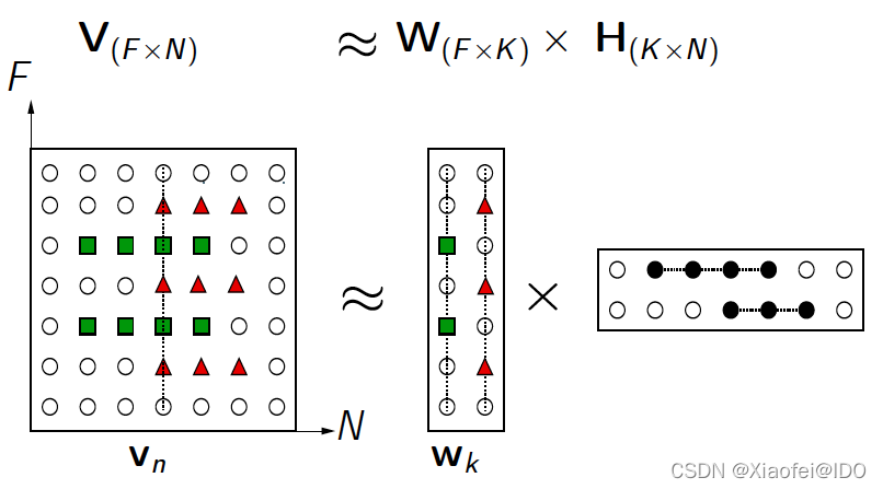
NMF(Non-negative matrix factorization)，即对于任意给定的一个非负矩阵 V，其能够寻找到一个非负矩阵 W 和一个非负矩阵 H，满足条件 $V=W\times H$，即将一个非负的矩阵分解为左右两个非负矩阵的乘积。
$$V=W\times H$$
其中，

• V矩阵中每一列代表一个观测(observation)，每一行代表一个特征(feature)；
• W矩阵称为基矩阵或特征的权重矩阵，代表每个特征对聚类结果的贡献度；
• H矩阵称为系数矩阵或样本的权重矩阵，代表每个样本对聚类结果的贡献度；
• 此时，用系数矩阵H代替原始矩阵，就可以实现对原始矩阵进行降维，得到数据特征的降维矩阵，从而减少存储空间。

图解如下：

二、python实现

在sklearn封装了NMF的实现，但是注意sklearn中输入数据的格式是（samples, features）：

from sklearn.decomposition import NMF
from sklearn.datasets import load_iris


X, _ = load_iris(True)

# can be used for example for dimensionality reduction, source separation or topic extraction
# 个人认为最重要的参数是n_components、alpha、l1_ratio、solver
nmf = NMF(n_components=2,  # k value,默认会保留全部特征
          init=None,  # W H 的初始化方法，包括'random' | 'nndsvd'(默认) |  'nndsvda' | 'nndsvdar' | 'custom'.
          solver='cd',  # 'cd' | 'mu'
          beta_loss='frobenius',  # {'frobenius', 'kullback-leibler', 'itakura-saito'}，一般默认就好
          tol=1e-4,  # 停止迭代的极限条件
          max_iter=200,  # 最大迭代次数
          random_state=None,
          alpha=0.,  # 正则化参数
          l1_ratio=0.,  # 正则化参数
          verbose=0,  # 冗长模式
          shuffle=False  # 针对"cd solver"
          )

# -----------------函数------------------------
print('params:', nmf.get_params())  # 获取构造函数参数的值，也可以nmf.attr得到，所以下面我会省略这些属性

# 下面四个函数很简单，也最核心，例子中见
nmf.fit(X)
W = nmf.fit_transform(X)
W = nmf.transform(X)
nmf.inverse_transform(W)
# -----------------属性------------------------
H = nmf.components_  # H矩阵
print('reconstruction_err_', nmf.reconstruction_err_)  # 损失函数值
print('n_iter_', nmf.n_iter_)  # 实际迭代次数

注意点：

• init参数中，nndsvd（默认）更适用于sparse factorization，其变体则适用于dense factorization.
• solver参数中，如果初始化中产生很多零值，Multiplicative Update (mu) 不能很好更新。所以mu一般不和nndsvd使用，而和其变体nndsvda、nndsvdar使用。
• solver参数中，cd只能优化Frobenius norm函数；而mu可以更新所有损失函数

图像特征提取

这里再举一个NMF在图像特征提取的应用，来自官方示例，根据我的需要改动了一些：

from time import time
from numpy.random import RandomState
import matplotlib.pyplot as plt
from sklearn.datasets import fetch_olivetti_faces
from sklearn import decomposition


n_row, n_col = 2, 3
n_components = n_row * n_col
image_shape = (64, 64)
rng = RandomState(0)

# #############################################################################
# Load faces data
dataset = fetch_olivetti_faces('./', True,
                               random_state=rng)
faces = dataset.data

n_samples, n_features = faces.shape

print("Dataset consists of %d faces, features is %s" % (n_samples, n_features))


def plot_gallery(title, images, n_col=n_col, n_row=n_row, cmap=plt.cm.gray):
    plt.figure(figsize=(2. * n_col, 2.26 * n_row))
    plt.suptitle(title, size=16)
    for i, comp in enumerate(images):
        plt.subplot(n_row, n_col, i + 1)
        vmax = max(comp.max(), -comp.min())
        plt.imshow(comp.reshape(image_shape), cmap=cmap,
                   interpolation='nearest',
                   vmin=-vmax, vmax=vmax)
        plt.xticks(())
        plt.yticks(())
    plt.subplots_adjust(0.01, 0.05, 0.99, 0.93, 0.04, 0.)


# #############################################################################
estimators = [
    ('Non-negative components - NMF',
     decomposition.NMF(n_components=n_components, init='nndsvda', tol=5e-3))
]

# #############################################################################
# Plot a sample of the input data

plot_gallery("First centered Olivetti faces", faces[:n_components])

# #############################################################################
# Do the estimation and plot it

for name, estimator in estimators:
    print("Extracting the top %d %s..." % (n_components, name))
    t0 = time()
    data = faces
    estimator.fit(data)
    train_time = (time() - t0)
    print("done in %0.3fs" % train_time)

    components_ = estimator.components_
    print('components_:', components_.shape, '\n**\n', components_)
    plot_gallery('%s - Train time %.1fs' % (name, train_time),
                 components_)
plt.show()

#---------------------------其他注释---------------------------
V矩阵：400*4096
W矩阵：400*6
H矩阵：6*4096