[基因遗传算法]进阶之三:sko.GA的实践TSP

参考资料:《VRP问题分类》

相关文章:
《[基因遗传算法]原理思想和python代码的结合理解之(一) :单变量》
《[基因遗传算法]进阶之二:最优规划问题–多种编码方式+多变量》

---

一. GA的用法

1.1 help(sko.GA)

GA(func, n_dim, size_pop=50, max_iter=200, prob_mut=0.001, lb=-1, ub=1, constraint_eq=(), 
constraint_ueq=(), precision=1e-07, early_stop=None)
 |  
 |  genetic algorithm
 |  
 |  Parameters
 |  ----------------
 |  func : function
 |      The func you want to do optimal 优化的目标函数
 |  n_dim : int
 |      number of variables of func目标函数的变量
 |  lb : array_like
 |      The lower bound of every variables of func每个变量的下限
 |  ub : array_like
 |      The upper bound of every variables of func每个变量的上限
 |  constraint_eq : tuple,
 |      equal constraint 等式约束
 |  constraint_ueq : tuple,
 |      unequal constraint不等式约束
 |  precision : array_like
 |      The precision of every variables of func 函数每个变量的精度
 |  size_pop : int
 |      Size of population种群数量
 |  max_iter : int
 |      Max of iter迭代次数
 |  prob_mut : float between 0 and 1
 |      Probability of mutation 突变概率

1.2 目标函数的书写

A. 单变量的书写

目标函数$y=10\cdot sin(5x)+7\cdot cos(4x)$

def aim(p):
    x= p[0]
    return -(10*np.sin(5*x)+7*np.cos(4*x))

B. 多变量的书写

目标函数$Z=2a+x^2-acos2\pi x+y^2-acos2\pi y$求最小值为例. $x\in [0,5],y\in [-5,5],a=10$.

def aim(p):
    a = 10
    pi = np.pi
    x,y=p
    return 2 * a + x ** 2 - a * np.cos(2 * pi * x) + y ** 2 - a * np.cos(2 * 3.14 * y)

C. 变量的范围

$x\in [0,5],y\in [-5,10]$
lb:low lb=[0,-5]
ub: upub=[5,10]

1.3 (不)等式约束的书写

二、实践TSP

这里应用的是GA_TSP算法.与GA算法不同.主要区分在目标函数的意义.

• GA的目标函数的变量是:(多个)自变量
• GA_TSP的目标函数的变量:是某个路径(环)

参考资料:《Python调用scikit-opt工具箱中的遗传算法求解TSP问题》
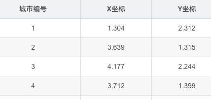
本案例以31个城市为例，假定31个城市的位置坐标如表1所列。寻找出一条最短的遍历31个城市的路径.城市列表见参考链接.

# 导入常用库
import numpy as np
import pandas as pd 
import matplotlib.pyplot as plt
from scipy import spatial #计算空间的
from sko.GA import GA 
from sko.GA import GA_TSP
from time import perf_counter
mpl.rcParams['font.sans-serif'] = ['SimHei']
mpl.rcParams['axes.unicode_minus'] = False

参考《scipy.spatial 距离计算模块》

A. 读取城市坐标,获得相关信息

读取.xlsx数据

file_name = 'cities.xlsx'#31座城市坐标数据文件
df = pd.read_excel(file_name)
points_coordinate=df.values 

读取.csv或.txt数据

file_name = 'data.csv'    #31座城市坐标数据文件
points_coordinate = np.loadtxt(file_name, delimiter=',')

计算城市间的欧式距离

num_points = points_coordinate.shape[0]
distance_matrix = spatial.distance.cdist(points_coordinate, points_coordinate, metric='euclidean')

☀️ 注意到,distance_matrix如果没有定义,则GA_TSP则执行的时候会报错.虽然GA_TSP中美有distance_matrix这个参数变量.

B.定义目标函数

即路线距离函数
路线routine举例为: 共31个城市的路线顺序.起点与终点的为同一个city.

def cal_total_distance(routine):
    '''计算总距离：输入路线,返回总距离.
    cal_total_distance(np.arange(num_points))
    '''
    num_points, = routine.shape
    return sum([distance_matrix[routine[i % num_points], routine[(i + 1) % num_points]] for i in range(num_points)])

C . 执行GA_TSP算法,输出结果

路径输出函数

def print_route(best_points):
    result_cur_best=[]
    for i in best_points:
        result_cur_best+=[i]
    for i in range(len(result_cur_best)):
        result_cur_best[i] += 1
    result_path = result_cur_best
    result_path.append(result_path[0])
    return result_path

执行算法

start=perf_counter()       #计时开始
# 执行遗传(GA)算法
ga_tsp = GA_TSP(func=cal_total_distance, n_dim=num_points, size_pop=300, max_iter=1000, prob_mut=1)   #调用工具箱

# 结果输出
best_points, best_distance = ga_tsp.run()
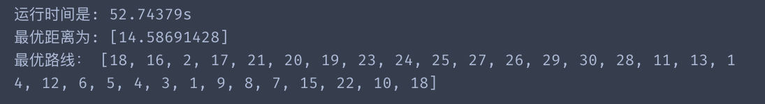
print("运行时间是: {:.5f}s".format(perf_counter()-start))   #计时结束
print("最优距离为:",best_distance)
print("最优路线：", print_route(best_points))

运行结果一:

缺city: 30
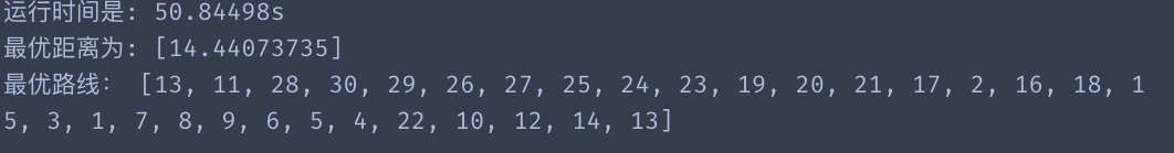
运行结果二:

缺city:0
运行结果三:

缺City:30
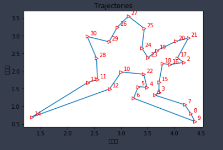
绘图展示

best_points_ = np.concatenate([best_points, [best_points[0]]])
#列表尾部添加起点城市
best_points_coordinate = points_coordinate[best_points_, :]#升维
fig1, ax1 = plt.subplots(1, 1)
ax1.set_title('Trajectories', loc='center')#轨迹图
line=ax1.plot(best_points_coordinate[:, 0], best_points_coordinate[:, 1], marker='>', mec='r', mfc='w')
for i in range(num_points):
    plt.text(best_points_coordinate[:, 0][i] + 0.05, best_points_coordinate[:, 1][i] + 0.05, str(best_points[i]+1), color='red')
ax1.set_xlabel("横坐标")
ax1.set_ylabel("纵坐标")

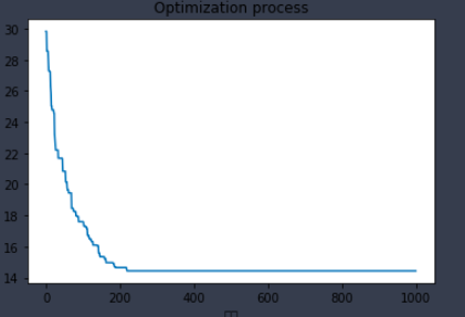
fig2, ax2 = plt.subplots(1, 1)
ax2.set_title('Optimization process', loc='center')#优化过程
ax2.plot(ga_tsp.generation_best_Y)
ax2.set_xlabel("代数")
ax2.set_ylabel("最优值")
plt.show()