


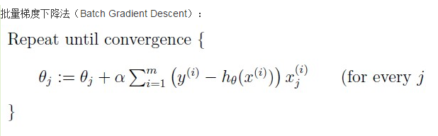
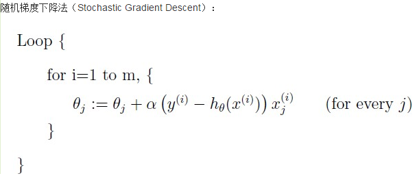
批梯度下降和随机梯度下降存在着一定的差异,主要是在theta的更新上,批量梯度下降使用的是将所有的样本都一批次的引入到theta的计算中,而随机梯度下降在更新theta时只是随机选择所有样本中的一个,然后对theta求导,所以随机梯度下降具有较快的速度,但是可能陷入局部最优解
以下是代码实现
#!usr/bin/python3
# coding:utf-8

# BGD 批梯度下降代码实现
# SGD 随机梯度下降代码实现
import numpy as np

import random


def batchGradientDescent(x, y, theta, alpha, m, maxInteration):
    x_train = x.transpose()
    for i in range(0, maxInteration):
        hypothesis = np.dot(x, theta)
        # 损失函数
        loss = hypothesis - y
        # 下降梯度
        gradient = np.dot(x_train, loss) / m
        # 求导之后得到theta
        theta = theta - alpha * gradient
    return theta


def stochasticGradientDescent(x, y, theta, alpha, m, maxInteration):
    data = []
    for i in range(4):
        data.append(i)
    x_train = x.transpose()
    for i in range(0, maxInteration):
        hypothesis = np.dot(x, theta)
        # 损失函数
        loss = hypothesis - y
        # 选取一个随机数
        index = random.sample(data, 1)
        index1 = index[0]
        # 下降梯度
        gradient = loss[index1] * x[index1]
        # 求导之后得到theta
        theta = theta - alpha * gradient
    return theta


def main():
    trainData = np.array([[1, 4, 2], [2, 5, 3], [5, 1, 6], [4, 2, 8]])
    trainLabel = np.array([19, 26, 19, 20])
    print(trainData)
    print(trainLabel)
    m, n = np.shape(trainData)
    theta = np.ones(n)
    print(theta.shape)
    maxInteration = 500
    alpha = 0.01
    theta1 = batchGradientDescent(trainData, trainLabel, theta, alpha, m, maxInteration)
    print(theta1)
    theta2 = stochasticGradientDescent(trainData, trainLabel, theta, alpha, m, maxInteration)
    print(theta2)
    return


if __name__ == "__main__":
    main()


 19万+
19万+

 被折叠的 条评论
为什么被折叠?
被折叠的 条评论
为什么被折叠?
 到【灌水乐园】发言


