时间序列--去趋势

转载于：https://blog.csdn.net/kylin_learn/article/details/85225400

https://machinelearningmastery.com/time-series-trends-in-python/

趋势是时间序列水平的长期增加或减少

有趋势的时间序列是非平稳的。

可以模拟确定的趋势。建模之后，它可以从时间系列数据集中去除。这就是时间序列去趋势。

该数据集有明显的上升趋势

差分法去趋势

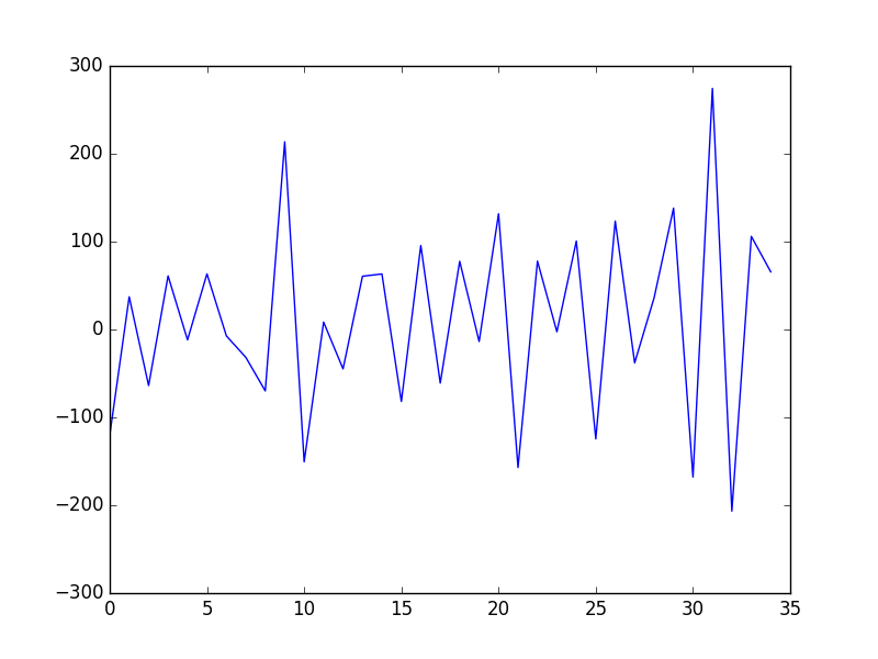
时间序列去趋势最简单的方法就是差分。

具体而言，在等时间步长的基础上，计算前一观察点和观察点之差构造出新的序列。

value(t) = observation(t) - observation(t-1)

1. from pandas import read_csv

2. from pandas import datetime

3. from matplotlib import pyplot

4.  

5. def parser(x):

6. return datetime.strptime('190'+x, '%Y-%m')

7.  

8. series = read_csv('shampoo-sales.csv', header=0, parse_dates=[0], index_col=0, squeeze=True, date_parser=parser)

9. X = series.values

10. diff = list()

11. for i in range(1, len(X)):

12. value = X[i] - X[i - 1]

13. diff.append(value)

14. pyplot.plot(diff)

15. pyplot.show()

去趋势之后变成这样

拟合模型去趋势

趋势通常可视化为一条直线穿过。

线性趋势可以用线性模型总结，非线性趋势可以用多项式或其它曲线拟合方法概括

例如，一个线性模型适用于时间指标预测。数据集如下所示︰

X,y

1,obs1

2,obs2

3,obs3

4,obs4

5,obs5

这个模型的预测将形成一条直线，可以作为该数据集的趋势线。这些预测也可以从原始时间序列中减去，以提供数据集的去趋势版本。

value(t) = observation(t) - prediction(t)

1. from pandas import read_csv

2. from pandas import datetime

3. from sklearn.linear_model import LinearRegression

4. from matplotlib import pyplot

5. import numpy

6.  

7. def parser(x):

8. return datetime.strptime('190'+x, '%Y-%m')

9.  

10. series = read_csv('shampoo-sales.csv', header=0, parse_dates=[0], index_col=0, squeeze=True, date_parser=parser)

11. # fit linear model

12. X = [i for i in range(0, len(series))]

13. X = numpy.reshape(X, (len(X), 1))

14. y = series.values

15. model = LinearRegression()

16. model.fit(X, y)

17. # calculate trend

18. trend = model.predict(X)

19. # plot trend

20. pyplot.plot(y)

21. pyplot.plot(trend)

22. pyplot.show()

23. # detrend

24. detrended = [y[i]-trend[i] for i in range(0, len(series))]

25. # plot detrended

26. pyplot.plot(detrended)

27. pyplot.show()

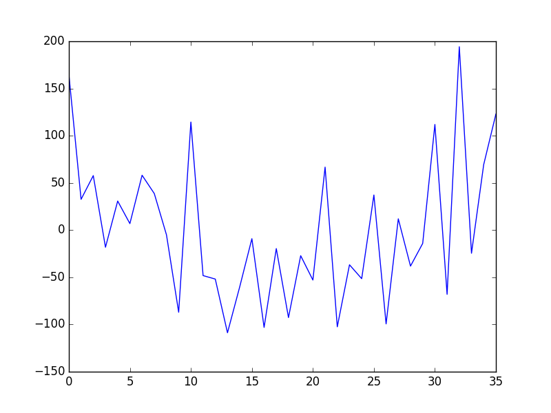
这里用了线性回归的model，当然也可以换成其他

在原始数据集（蓝色）上绘制趋势线 （绿色）

下一步，原始数据集减去这一趋势，然后绘制结果，结果为去趋势数据集。

进一步深入：http://www.ltrr.arizona.edu/webhome/dmeko/notes_7.pdf