Matplotlib Toolkits：三维绘图工具包matplotlib.mplot3d

http://blog.csdn.net/pipisorry/article/details/40008005

Matplotlib mplot3d 工具包简介

The mplot3d toolkit adds simple 3D plotting capabilities to matplotlib by supplying an axes object that can create a 2D projection of a 3D scene. The resulting graph will have the same look and feel as regular 2D plots.

创建Axes3D对象

An Axes3D object is created just like any other axes using the projection=‘3d’ keyword. Create a new matplotlib.figure.Figure and add a new axes to it of type Axes3D:
import matplotlib.pyplot as plt
from mpl_toolkits.mplot3d import Axes3D
fig = plt.figure()
ax = fig.add_subplot(111, projection=’3d’)
New in version 1.0.0: This approach is the preferred method of creating a 3D axes.
Note: Prior to version 1.0.0, the method of creating a 3D axes was di erent. For those using older versions of matplotlib, change ax = fig.add_subplot(111, projection=’3d’) to ax = Axes3D(fig).

要注意的地方

Axes3D展示三维图形时，其初始视图中x,y轴与我们一般看的视图（自己画的时候的视图）是反转的，matlab也是一样。

可以通过设置初始视图来改变角度：ax.view_init(30, 35)

Note: 不过这样图形可能会因为旋转而有阴影，也可以通过代码中XY轴互换来实现视图中XY互换。不知道有没有其它方法，如matlab中就有surf(x,y,z);set(gca,'xdir','reverse','ydir','reverse')这样命令来实现这个功能[关于matlab三维图坐标轴原点位置的问题]。

lz总结绘制三维图形一般流程

创建Axes3D对象

fig = plt.figure()
ax = Axes3D(fig)

再进行坐标范围设定什么的（可选）

# 计算坐标极限值
xs = list(itertools.chain.from_iterable([xi[0] for xi in x]))
x_max, x_min = max(xs), min(xs)
ys = list(itertools.chain.from_iterable([xi[1] for xi in x]))
y_max, y_min = max(ys), min(ys)
zs = list(itertools.chain.from_iterable([xi[2] for xi in x]))
z_max, z_min = max(zs), min(zs)
margin = 0.1

再进行绘制，如

plt.scatter(x_new[0], x_new[1], c='r', marker='*', s=50, label='new x')
ax.scatter(xs, ys, zs, c=c, marker=marker, s=50, label=label)
ax.plot_surface(X, Y, Z, rstride=1, cstride=1, label='Discrimination Interface')

再进行一些坐标什么的设置

# 设置图形展示效果
ax.set_xlim(x_min - margin, x_max + margin)
ax.set_ylim(y_min - margin, y_max + margin)
ax.set_zlim(z_min - margin, z_max + margin)
ax.set_xlabel('x')
ax.set_ylabel('y')
ax.set_zlabel('z')
ax.legend(loc='lower right')
ax.set_title('Plot of class0 vs. class1')
ax.view_init(30, 35)

最后显示出来

plt.show()

皮皮blog

绘制不同三维图形

Line plots线图

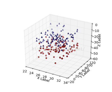
Scatter plots散点图

Axes3D.scatter(xs, ys, zs=0, zdir=u'z', s=20, c=u'b', depthshade=True, *args, **kwargs)

Create a scatter plot

Argument	Description
xs, ys	Positions of data points.
zs	Either an array of the same length as xs andys or a single value to place all points inthe same plane. Default is 0.
zdir	Which direction to use as z (‘x’, ‘y’ or ‘z’)when plotting a 2D set.
s	size in points^2. It is a scalar or an array of thesame length as x andy.
c	a color. c can be a single color format string, or asequence of color specifications of lengthN, or asequence ofN numbers to be mapped to colors using thecmap andnorm specified via kwargs (see below). Notethatc should not be a single numeric RGB or RGBAsequence because that is indistinguishable from an arrayof values to be colormapped.c can be a 2-D array inwhich the rows are RGB or RGBA, however.
depthshade	Whether or not to shade the scatter markers to givethe appearance of depth. Default isTrue.

Keyword arguments are passed on to scatter(). Returns a Patch3DCollection Note: scatter ( x, y, s=20, c=u'b', marker=u'o', cmap=None, norm=None, vmin=None, vmax=None, alpha=None, linewidths=None, verts=None, **kwargs )

Wireframe plots线框图

Surface plots曲面图

参数

x, y, z: x,y,z轴对应的数据。注意z的数据的z.shape是(len(y), len(x))，不然会报错：ValueError: shape mismatch: objects cannot be broadcast to a single shape

rstride    Array row stride (step size), defaults to 10
cstride    Array column stride (step size), defaults to 10

示例1：

import numpy as np
import matplotlib.pyplot as plt
from mpl_toolkits.mplot3d import Axes3D

fig = plt.figure()
ax = Axes3D(fig)
X = np.arange(-4, 4, 0.25)
Y = np.arange(-4, 4, 0.25)
X, Y = np.meshgrid(X, Y)
R = np.sqrt(X**2 + Y**2)
Z = np.sin(R)

ax.plot_surface(X, Y, Z, rstride=1, cstride=1, cmap=plt.cm.hot)
ax.contourf(X, Y, Z, zdir='z', offset=-2, cmap=plt.cm.hot)
ax.set_zlim(-2,2)

# savefig('../figures/plot3d_ex.png',dpi=48)
plt.show()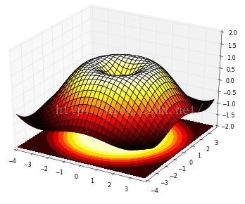

结果图形输出：

示例2：

import numpy as np
import matplotlib.pyplot as plt
from mpl_toolkits.mplot3d import Axes3D

fig = plt.figure()
ax = Axes3D(fig)

x = np.arange(0, 200)
y = np.arange(0, 100)
x, y = np.meshgrid(x, y)
z = np.random.randint(0, 200, size=(100, 200))%3
print(z.shape)

# ax.scatter(x, y, z, c='r', marker='.', s=50, label='')
ax.plot_surface(x, y, z,label='')
plt.show()

[surface-plots]

[Matplotlib tutorial - 3D Plots]

Tri-Surface plots三面图

Contour plots等高线图

Filled contour plots填充等高线图

Polygon plots多边形图

Axes3D.add_collection3d(col, zs=0, zdir=u'z')

Add a 3D collection object to the plot.

2D collection types are converted to a 3D version bymodifying the object and adding z coordinate information.

Supported are:

• PolyCollection
• LineColleciton
• PatchCollection

绘图原理是：设置好多面体（如正文体）的顶点坐标和所有面对应的顶点，加上一些属性（如颜色、宽度、透明度）

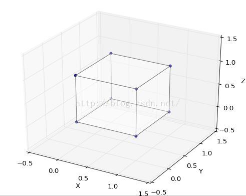
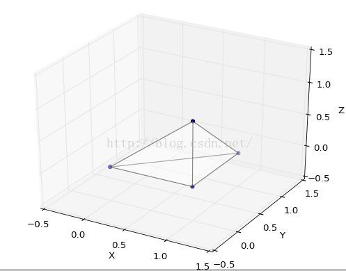
绘制正方体和四面体示例

#!/usr/bin/env python
# -*- coding: utf-8 -*-
"""
__title__ = ''
__author__ = '皮'
__mtime__ = '9/27/2015-027'
__email__ = 'pipisorry@126.com'
"""
import matplotlib.pyplot as plt
from mpl_toolkits.mplot3d.art3d import Poly3DCollection

fig = plt.figure()
ax = fig.gca(projection='3d')


# 正文体顶点和面
verts = [(0, 0, 0), (0, 1, 0), (1, 1, 0), (1, 0, 0), (0, 0, 1), (0, 1, 1), (1, 1, 1), (1, 0, 1)]
faces = [[0, 1, 2, 3], [4, 5, 6, 7], [0, 1, 5, 4], [1, 2, 6, 5], [2, 3, 7, 6], [0, 3, 7, 4]]
# 四面体顶点和面
# verts = [(0, 0, 0), (1, 0, 0), (1, 1, 0), (1, 0, 1)]
# faces = [[0, 1, 2], [0, 1, 3], [0, 2, 3], [1, 2, 3]]
# 获得每个面的顶点
poly3d = [[verts[vert_id] for vert_id in face] for face in faces]
# print(poly3d)

# 绘制顶点
x, y, z = zip(*verts)
ax.scatter(x, y, z)
# 绘制多边形面
ax.add_collection3d(Poly3DCollection(poly3d, facecolors='w', linewidths=1, alpha=0.3))
# ax.add_collection3d(Line3DCollection(poly3d, colors='k', linewidths=0.5, linestyles=':'))

 # 设置图形坐标范围ax.set_xlabel('X')ax.set_xlim3d(-0.5, 1.5)ax.set_ylabel('Y')ax.set_ylim3d(-0.5, 1.5)ax.set_zlabel('Z')ax.set_zlim3d(-0.5, 1.5)plt.show()

绘制结果截图

  

[Transparency for Poly3DCollection plot in matplotlib]

Bar plots条形图

2D plots in 3D三维图中的二维图

Text文本图

Subplotting子图

皮皮blog

matplotlib.mplot3d绘图实例

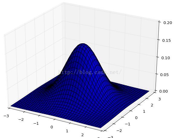
matplotlib绘制2维高斯分布

import matplotlib.pyplot as plt
from mpl_toolkits.mplot3d import Axes3D
fig = plt.figure()
ax = Axes3D(fig)
rv = stats.multivariate_normal([0, 0], cov=1)

x, y = np.mgrid[-3:3:.15, -3:3:.15]
ax.plot_surface(x, y, rv.pdf(np.dstack((x, y))), rstride=1, cstride=1)
ax.set_zlim(0, 0.2)

# savefig('../figures/plot3d_ex.png',dpi=48)
plt.show()

matplotlib绘制平行z轴的平面

（垂直xy平面的平面）

方程：0*Z + A[0]X + A[1]Y + A[-1] = 0

X = np.arange(x_min - margin, x_max + margin, 0.05)
Z = np.arange(z_min - margin, z_max + margin, 0.05)
X, Z = np.meshgrid(X, Z)
Y = -1 / A[1] * (A[0] * X + A[-1])
ax.plot_surface(X, Y, Z, rstride=1, cstride=1, label='Discrimination Interface')

from:http://blog.csdn.net/pipisorry/article/details/40008005

ref:mplot3d tutorial(inside source code)

mplot3d API

[mplot3d¶]