


NN概述
神经网络最主要的作用是作为提取特征的工具,最终的分类并不是作为主要核心。
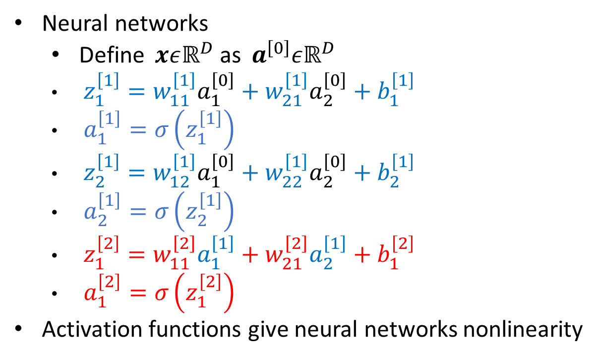
人工神经网络也称为多层感知机,相当于将输入数据通过前面多个全连接层网络将原输入特征进行了一个非线性变换,将变换后的特征拿到最后一层的分类器去分类。
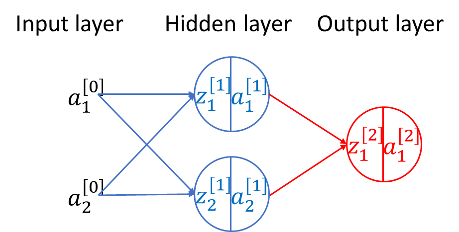
神经网络是由多个神经元组成的拓扑结构,由多个层排列组成,每一层又堆叠了多个神经元。通常包括输入层,N个隐藏层,和输出层组成。
1、前馈神经网络具有很强的拟合能力,常见的连续非线性函数都可以用前馈 神经网络来近似.
2、根据通用近似定理,神经网络在某种程度上可以作为一个“万能”函数来使 用,可以用来进行复杂的特征转换,或逼近一个复杂的条件分布
3、一般是通过经验风险最小化和正则化来 进行参数学习.因为神经网络的强大能力,所以容易在训练集上过拟合.
4、神经网络的优化问题是一个非凸优化问题,而且可能面临梯度消失的问题。
NN原理
代码部分
部分关键代码
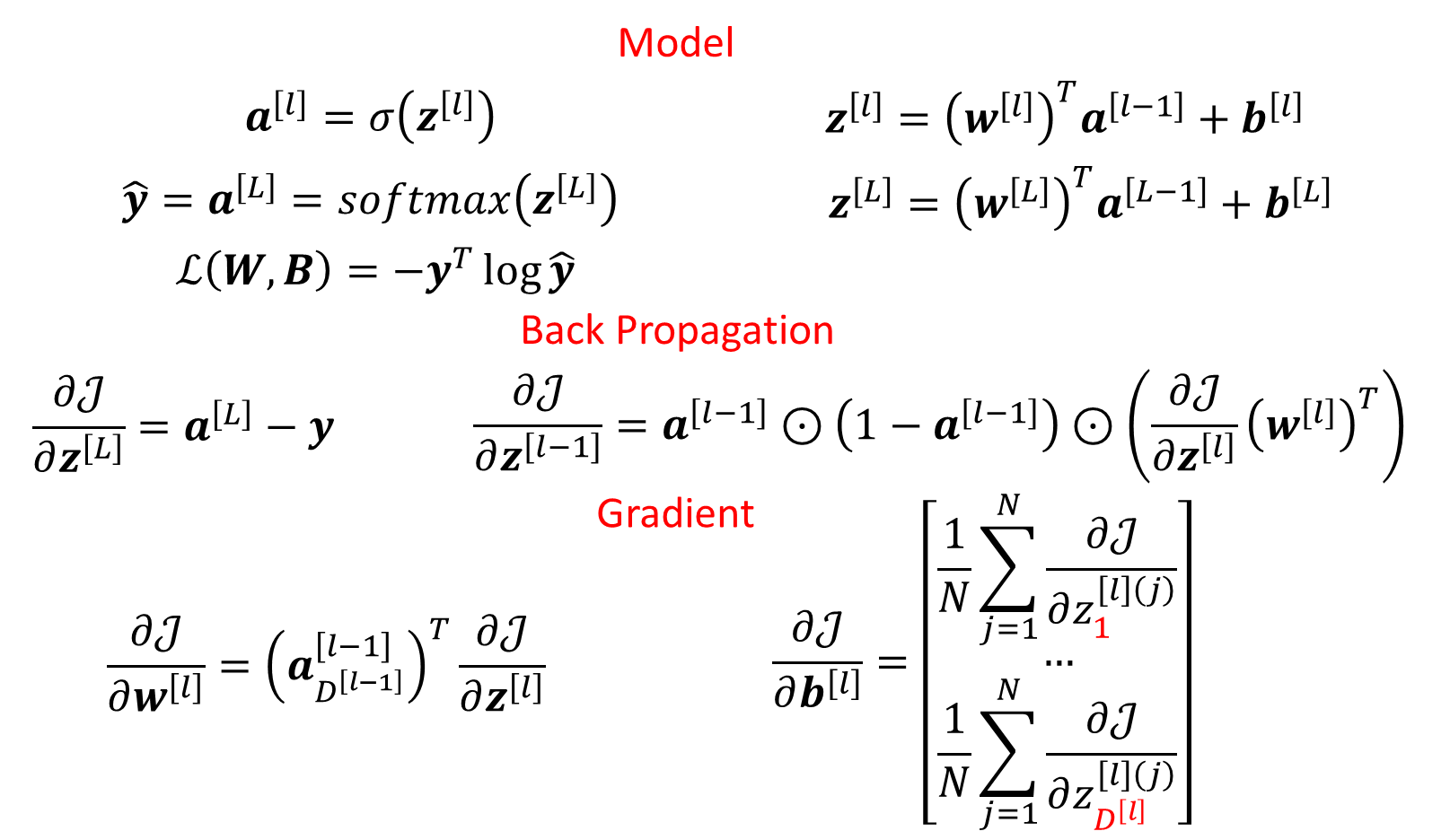
- 前向传播
      X = np.atleast_2d(X)
      A[0] = X
      A[1] = np.dot(A[0], W[0]) + B[0]
      A[2] = np.dot(A[1], W[1]) + B[1]
      A[2] = np.exp(A[2]) / (np.expand_dims(np.sum(np.exp(A[2]), axis=1), axis=1) * np.ones((1, (A[2]).shape[1])))
- 反向传播(更新,全部用矩阵乘法速度max)
      error = Y - A[2]
      deltas = [error]
      layer_num = len(a) - 2  # 导数第二层开始
      for j in range(layer_num, 0, -1):
            deltas.append(deltas[-1].dot(W[j].T))  # 误差的反向传播
      deltas[-1][a[1]==0]=0
      deltas.reverse()
      for i in range(len(W)):  # 正向更新权值
            layer = np.atleast_2d(a[i])
            delta = np.atleast_2d(deltas[i])

            dW[i] = layer.T.dot(delta)
            dB[i] =  deltas[i]
代码汇总
# -*- coding: utf-8 -*-
import numpy as np
import matplotlib.pyplot as plt
# Utilities
def onehotEncoder(Y, ny):
return np.eye(ny)[Y]
def sigmoid(x): # 激活函数采用Sigmoid
return 1 / (1 + np.exp(-x))
def sigmoid_derivative(x): # Sigmoid的导数
return sigmoid(x) * (1 - sigmoid(x))
def softmax(z):
hat_z = [0]*len(z)
for i in range(len(z)):
hat_z[i] = np.exp(z[i])/np.sum(np.exp(z))
return hat_z
# Xavier Initialization
def initWeights(M):
l = len(M)
W = []
B = []
for i in range(1, l):
W.append(np.random.randn(M[i - 1], M[i]))
B.append(np.random.randn(1, M[i]))
return W, B
# Forward propagation
def networkForward(X, W, B):
l = len(W)
A = [None for i in range(l + 1)]
##### Calculate the output of every layer A[i], where i = 0, 1, 2, ..., l
X = np.atleast_2d(X)
A[0] = X
A[1] = np.dot(A[0], W[0]) + B[0]
A[2] = np.dot(A[1], W[1]) + B[1]
A[2] = np.exp(A[2]) / (np.expand_dims(np.sum(np.exp(A[2]), axis=1), axis=1) * np.ones((1, (A[2]).shape[1])))
return A
# --------------------------
# Backward propagation
def networkBackward(Y, A, W):
l = len(W)
dW = [None for i in range(l)]
dB = [None for i in range(l)]
a = A
error = Y - A[2]
deltas = [error]
layer_num = len(a) - 2 # 导数第二层开始
for j in range(layer_num, 0, -1):
deltas.append(deltas[-1].dot(W[j].T)) # 误差的反向传播
deltas[-1][a[1]==0]=0
deltas.reverse()
for i in range(len(W)): # 正向更新权值
layer = np.atleast_2d(a[i])
delta = np.atleast_2d(deltas[i])
dW[i] = layer.T.dot(delta)
dB[i] = deltas[i]
return dW, dB
#--------------------------
#Update weights by gradient descent
def updateWeights(W, B, dW, dB, lr):
l = len(W)
for i in range(l):
W[i] = W[i] + lr*dW[i]
B[i] = B[i] + lr*dB[i]
return W, B
#Compute regularized cost function
def cost(A_l, Y, W):
n = Y.shape[0]
c = -np.sum(Y*np.log(A_l)) / n
return c
def train(X, Y, M, lr = 0.0001, iterations = 3000):
costs = []
W, B = initWeights(M)
for i in range(iterations):
A = networkForward(X, W, B)
c = cost(A[-1], Y, W)
# print(A[-1])
dW, dB = networkBackward(Y, A, W)
W, B = updateWeights(W, B, dW, dB, lr)
if i % 100 == 0:
print("Cost after iteration %i: %f" %(i, c))
costs.append(c)
test(Y, X, W, B)
# l = np.random.randint(0,X.shape[0])
# p, _ = predict_t(X[l], W, B, Y)
# print('模型识别为:', p,"实际为:",Y[l])
return W, B, costs
def predict(X, W, B, Y):
Y_out = np.zeros([X.shape[0], Y.shape[1]])
A = networkForward(X, W, B)
idx = np.argmax(A[-1], axis=1)
Y_out[range(Y.shape[0]),idx] = 1
return Y_out
def test(Y, X, W, B):
Y_out = predict(X, W, B, Y)
# print(Y_out)
acc = np.sum(Y_out*Y) / Y.shape[0]
print("Training accuracy is: %f" %(acc))
return acc
iterations = 5000###### Training loops
lr = 0.0001###### Learning rate
data = np.load("data.npy")
X = data[:,:-1]
Y = data[:,-1].astype(np.int32)
(n, m) = X.shape
Y = onehotEncoder(Y, 10)
M = [400, 25, 10]
W, B, costs = train(X, Y, M, lr, iterations)
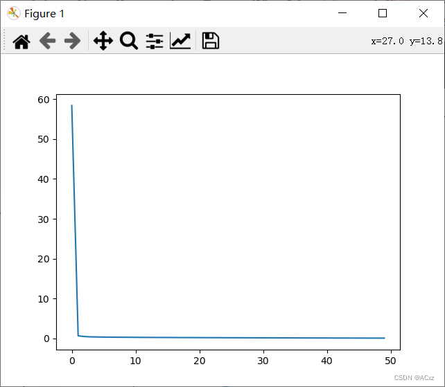
plt.figure()
plt.plot(range(len(costs)), costs)
plt.show()
test(Y, X, W, B)
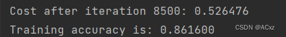
结果截图
](https://img-blog.csdnimg.cn/cdb40b511905493095158f262af716d4.png)


 3651
3651


 被折叠的 条评论
为什么被折叠?
被折叠的 条评论
为什么被折叠?
 到【灌水乐园】发言


