《Py机器学习》—朴素贝叶斯

        朴素贝叶斯——一种有监督的学习算法，基于样本特征之间互相“独立”的这个朴素假设，不用考虑样本特征之间的关系，效率很高。适应于样本数量比较说

 

1.普通的朴素贝叶斯

import numpy as np
#导入输入数组和输出数组
X = np.array([[0,1,0,1],
              [1,1,1,0],
              [0,1,1,0],
              [0,0,0,1],
              [0,1,1,0],
              [0,1,0,1],
              [1,0,0,1]])
y = np.array([0,1,1,0,1,0,0])
#统计当结果为0或1时，各个特征为1的个数
counts = {}
for lable in np.unique(y):
    counts[lable] = X[y == lable].sum(axis = 0)
#打印计数结果
print("feature counts:\n{}".format(counts))

        运行结果：

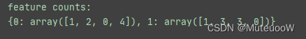
        表示为当结果（y）是0的时候，输入样本特征为1的个数是1，2，0，4个。这将成为朴素贝叶斯的推理标准。 

        下面用刚才的模型进行一下预测：

import numpy as np
from sklearn.naive_bayes import BernoulliNB  #导入贝叶斯拟合模型
#导入输入数组和输出数组
X = np.array([[0,1,0,1],
              [1,1,1,0],
              [0,1,1,0],
              [0,0,0,1],
              [0,1,1,0],
              [0,1,0,1],
              [1,0,0,1]])
y = np.array([0,1,1,0,1,0,0])
#使用贝叶斯拟合工具
clf = BernoulliNB()
clf.fit(X,y)
Next_Day = [[0,0,0,0]]
pre = clf.predict(Next_Day)
#进行判断
if pre == 1:
    print("预测结果为1")
else:
    print("预测结果为0")

        预测结果的概率：

#预测准确率
print(clf.predict_proba(Next_Day))

        显示结果如下，表示结果为1的概率76%，结果为0的概率23%

 2.各种贝叶斯

2.1贝努利朴素贝叶斯

        适用场景：符合“0-1分布”或“二项分布的“数据集。即只有0，1的分布

        用贝叶斯验证一下bool分布

from sklearn.datasets import make_blobs #导入数据集生成工具
from sklearn.model_selection import train_test_split #导入数据集拆分工具
from sklearn.naive_bayes import BernoulliNB

X,y = make_blobs(n_samples=500 ,centers=5 ,random_state= 6) #生成数据
X_train,X_test,y_train,y_test = train_test_split(X,y,random_state=6) #拆分数据
#进行拟合
nb = BernoulliNB()
nb.fit(X_train,y_train)
#打印模型得分
print("模型得分：{:.3f}".format(nb.score(X_test,y_test)))

         发现模型的得分只有0.416

        下面图解一下分类情况，运行代码：

from sklearn.datasets import make_blobs #导入数据集生成工具
from sklearn.model_selection import train_test_split #导入数据集拆分工具
from sklearn.naive_bayes import BernoulliNB
import matplotlib.pyplot as plt #导入作图工具
import numpy as np
import matplotlib.colors

X,y = make_blobs(n_samples=500 ,centers=5 ,random_state= 6) #生成数据
X_train,X_test,y_train,y_test = train_test_split(X,y,random_state=6) #拆分数据
#进行拟合
nb = BernoulliNB()
nb.fit(X_train,y_train)
#打印模型得分
print("模型得分：{:.3f}".format(nb.score(X_test,y_test)))

#限定横轴和纵轴的最大值
x_min,x_max = X[:,0].min()-0.5 , X[:,0].max()+0.5
y_min,y_max = X[:,1].min()-0.5 , X[:,1].max()+0.5

# #用不同的背景色表示不同的分类
xx,yy = np.meshgrid(np.arange(x_min, x_max, .02),
                     np.arange(y_min, y_max, .02))
z = nb.predict(np.c_[(xx.ravel(),yy.ravel())]).reshape(xx.shape)
plt.pcolormesh(xx,yy,z,shading='auto',cmap=plt.cm.Pastel1)  #****注意这里，py3.3版本之后要加上shading='auto'，否则报错

#将训练集和测试集用散点图表示
plt.scatter(X_train[:,0],X_train[:,1],c = y_train,cmap = plt.cm.Reds,edgecolors='k')
plt.scatter(X_test[:,0],X_test[:,1],c = y_test,cmap = plt.cm.Reds,marker='*',edgecolors='k')
plt.xlim(xx.min(),xx.max())
plt.ylim(yy.min(),yy.max())
#定义图题
plt.title('Llassifier:BernoulliNB')
plt.show()

        显示图像如下。利用x=0和y=0分成四个象限，如果特征值1和特征值2都大于0，则归为1类；如果特征值1和特征值2都小于0，归为另一类；其余都归为第三类。（真的是非常粗糙的归类呢）

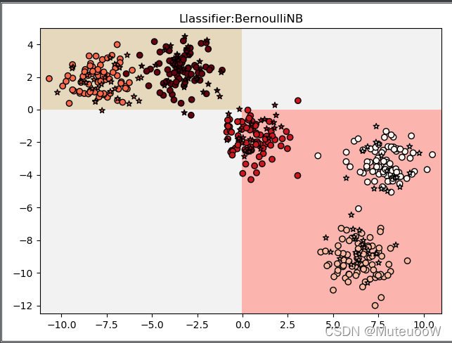
         得分非常低，这个时候就要考虑用别的分类啦

2.2.高斯朴素贝叶斯

        适用场景：假设样本符合高斯分布，即正态分布

        下面用高斯分布再验证一下我们刚才生成的数据集，只需要修改两处：

from sklearn.naive_bayes import GaussianNB #导入高斯分布

nb = GaussianNB()  #利用高斯拟合

        模型得分0.984，准确率高达98.7%，说明生成的数据集几乎符合高斯分布！

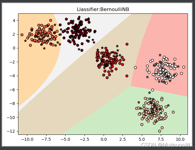
         高斯分布可以胜任大部分的分类任务，因为大量现象都是呈现正态分布

2.3.多项式朴素贝叶斯 

        适用场景：用于拟合多项式分布的非负离散数据特征集

        多项式分布：可以理解为扔骰子，每一次扔出的结果都有可能是1-6，那么如果扔n次，每个面朝上的次数的分布情况就是多项式分布

【注】多项式贝叶斯不可像前两个一样只通过修改两个部分就实现，还需要对数据进行处理

        用多项式贝叶斯再拟合一下刚才的数据集：

from sklearn.datasets import make_blobs
from sklearn.model_selection import train_test_split
from sklearn.naive_bayes import MultinomialNB
import matplotlib.pyplot as plt
import numpy as np
from sklearn.preprocessing import MinMaxScaler #数据预处理工具

X,y = make_blobs(n_samples=500 ,centers=5 ,random_state= 6)
X_train,X_test,y_train,y_test = train_test_split(X,y,random_state=6)
#预处理数据
scaler = MinMaxScaler()
scaler.fit(X_train)
X_train_scaled = scaler.transform(X_train)
X_test_scaled = scaler.transform(X_test)
#拟合预处理过的数据
nb = MultinomialNB()
nb.fit(X_train_scaled,y_train)
#打印模型得分
print("模型得分：{:.3f}".format(nb.score(X_test_scaled,y_test)))

#绘图
x_min,x_max = X[:,0].min()-0.5 , X[:,0].max()+0.5
y_min,y_max = X[:,1].min()-0.5 , X[:,1].max()+0.5
xx,yy = np.meshgrid(np.arange(x_min, x_max, .02),
                     np.arange(y_min, y_max, .02))
z = nb.predict(np.c_[(xx.ravel(),yy.ravel())]).reshape(xx.shape)
plt.pcolormesh(xx,yy,z,shading='auto',cmap=plt.cm.Pastel1)
plt.scatter(X_train[:,0],X_train[:,1],c = y_train,cmap = plt.cm.Reds,edgecolors='k')
plt.scatter(X_test[:,0],X_test[:,1],c = y_test,cmap = plt.cm.Reds,marker='*',edgecolors='k')
plt.xlim(xx.min(),xx.max())
plt.ylim(yy.min(),yy.max())
plt.show()

        观察图像可知，这个模型并不适合这个数据集：

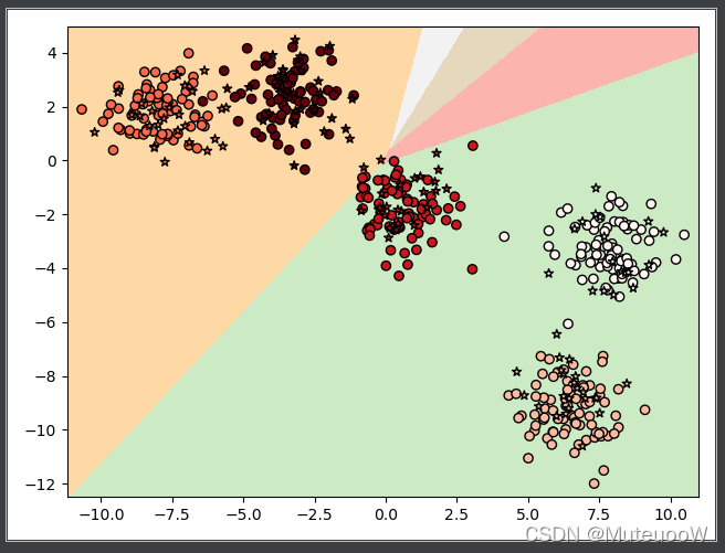
         多项式贝叶斯的典型应用：对转化为向量后的文本数据进行分类

2.4.贝叶斯应用一下——拟合自带的乳腺癌数据

from sklearn.datasets import load_breast_cancer  #导入肿瘤数据集
from sklearn.model_selection import train_test_split
from sklearn.naive_bayes import GaussianNB

cancer = load_breast_cancer()
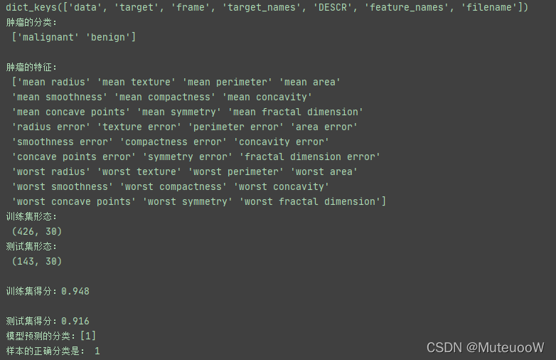
print(cancer.keys())  #打印这个数据的键值
print('肿瘤的分类：\n',cancer['target_names'])
print('\n肿瘤的特征：\n',cancer['feature_names'])

X,y = cancer.data,cancer.target #
X_train,X_test,y_train,y_test = train_test_split(X,y,random_state=30)
print('训练集形态：\n',X_train.shape) #查看训练集和测试集各有多少组数据，并且有多少个特征
print('测试集形态：\n',X_test.shape) #结果表示：训练集426个，测试集143个，特征数量都是30
#建模，测试一下分数
gnb = GaussianNB()
gnb.fit(X_train,y_train)
print('\n训练集得分：{:.3f}'.format(gnb.score(X_train,y_train)))
print('\n测试集得分：{:.3f}'.format(gnb.score(X_test,y_test)))
#选择第312个数据做一下测试
print('模型预测的分类：{}'.format(gnb.predict([X[312]])))
print('样本的正确分类是：',y[312])

输出结果如下：

 【注】这里本来想用上面的绘图程序画个图，但是报错显示：ValueError: operands could not be broadcast together with shapes (1692603,2) (30,) 。这时因为上面只能画出二维，但是本数据30维，所以不会绘图

3.学习曲线

        概念：随着数据集样本数量增加，模型的得分情况

from sklearn.datasets import load_breast_cancer
from sklearn.model_selection import train_test_split
from sklearn.naive_bayes import GaussianNB
import matplotlib.pyplot as plt
import numpy as np
from sklearn.model_selection import learning_curve #导入学习曲线库
from sklearn.model_selection import ShuffleSplit #导入随机拆分工具
cancer = load_breast_cancer()
X,y = cancer.data,cancer.target #
X_train,X_test,y_train,y_test = train_test_split(X,y,random_state=30)
gnb = GaussianNB()
gnb.fit(X_train,y_train)

#定义一个函数绘制学习曲线
def plot_learning_curve(estimator,title,X,y,ylim = None,cv = None,
                        n_jobs = 1,train_sizes = np.linspace(.1,1.0,5)):
    plt.figure()
    plt.title(title)
    if ylim is not None:
        plt.ylim(*ylim)
    #设定横轴坐标
    plt.xlabel("Training exanples")
    #设定纵轴坐标
    plt.ylabel("Score")
    train_sizes,train_scores,test_scores = learning_curve(
        estimator,X,y,cv = cv,n_jobs=n_jobs,train_sizes=train_sizes)
    train_scores_mean = np.mean(train_scores,axis=1)
    test_scores_mean = np.mean(test_scores,axis=1)
    plt.grid()
    plt.plot(train_sizes,train_scores_mean,'o-',color="r",label = "Training score")
    plt.plot(train_sizes,test_scores_mean,'o-',color="g",label = "Cross-validation score")
    plt.legend(loc = "lower right")
    return plt

#设置标题
title = "Learning Curves"
#设定拆分数量
cv = ShuffleSplit(n_splits=100,test_size=0.2,random_state=0)
#设定模型为高斯朴素贝叶斯
estimator = GaussianNB()
#调用我们调好的函数
plot_learning_curve(estimator,title,X,y,ylim=(0.9,1.01),cv=cv,n_jobs=4)
#显示图片
plt.show()

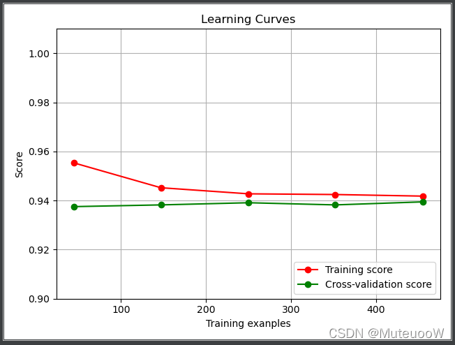
         如果样本数量比较少的话，可以考虑朴素贝叶斯