论文阅读 IEEE TITS 2023 | 4D High-Resolution Imagery of Point Clouds for Automotive mmWave Radar

原文链接： https://mp.weixin.qq.com/s?__biz=Mzg4MjgxMjgyMg==&mid=2247486184&idx=1&sn=c3d6c19d03d519906fc606ec367af4f2&chksm=cf51b811f82631078407c3a8740932d42a1e0dd315416375721f49150c33dfa9d68f02bc7337#rd

论文阅读 IEEE TITS 2023 | 4D High-Resolution Imagery of Point Clouds for Automotive mmWave Radar

毫米波成像论文阅读笔记 | IEEE TITS, 2023 4D High-Resolution Imagery of Point Clouds for Automotive mmWave Radar

@article{jiang20234d,
  title={4D High-Resolution Imagery of Point Clouds for Automotive mmWave Radar},
  author={Jiang, Mengjie and Xu, Gang and Pei, Hao and Feng, Zeyun and Ma, Shuai and Zhang, Hui and Hong, Wei},
  journal={IEEE Transactions on Intelligent Transportation Systems},
  year={2023},
  publisher={IEEE}
}

0 Abstract

• 4D mmwave radar面临的问题：

  • too sparse: due to the limitation of Doppler and angle resolutions

• 本文贡献：

  • 提出了一种高doppler and angle resolution的algorithm

  • 1 高Doppler resolution with high-dynamic:

    ✅ propose a novel velocity ambiguity resolution algorithm

    🚩 using a dual pulse repetition frequency (dual-PRF) waveform design + embedded in an time-division multiplexing & Doppler-division multiplexing MIMO (TDM-DMM-MIMO) framework

  • 2 高Angular resolution:

    ✅ propose a complex-valued deep convolution network (CV-DCN) of DOA-SR estimation (with only one single frame)

    🚩 apply a spatial smoothing operator on array data as input

    🚩 CV-DCN: end-to-end spectrum extraction

• 实验结果：

  • 1 confirm the effectiveness of the proposed algorithm
  • 2 4D high resolution imagery of PCD by experiments in the parking lot

1 Introduction

4D mmwave radar 应用前景很广

1.1 Introduction of Related Work

MIMO + 多芯片级联 方案 面临的问题：

• 1 如何优化正交波形设计
• 2 高动态高分辨率速度测量
• 3 高分辨率DOA估计

$\Rightarrow$ 下面分别进行介绍

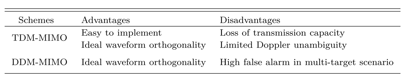
1.1.1 Orthogonal Waveform Design

• TDM 时分复用
  • 优点：简单、正交性好
  • 缺点：牺牲了MIMO transmission capability + PRI (Pulse repetition interval)
• CDM 码分复用
  • 多个TX同时发射波形，但是需要使用不同的random codes进行调制
  • 优点：MIMO传输容量 is efficiently exploited
  • 缺点：high-level interferences are inevitable in the Doppler domain ( 因为不同coded waveforms之间的非理想正交性)
• DDM 多普勒分复用
  • the transmitted waveforms are modulated by multiple sets of linear phase codes
  • these codes are distinct for each transmitted waveform and switched between pulses
  • 优点：completely separated in the Doppler domain with various Doppler offsets
  • 缺点：难以identifying true targets from ghost targets in the Doppler domain, particularly in multi-target scenarios

1.1.2 Velocity Ambiguity Resolution

• 速度模糊：
  • 当目标的多普勒频率超过脉冲重复频率（PRF）的一个周期时，就会出现多普勒模糊
• TDM-MIMO中的固有矛盾：
  • 最大无歧义速度与发射器的数量成反比地减小
• 解决上述问题的方案：
  • 具有不同PRF和中国剩余定理（CRT的框架 ([14])
  • 一种基于不规则脉冲间隔和稀疏信号处理的类似算法 ([17])
  • 基于相位编码方案，利用每个峰值的功率来分离传输信号，从而解决速度模糊问题 ([18,19]) $\Rightarrow$ 但当目标在范围内重叠时，RD图像严重恶化
  • 用基于 TDM 方案 [21] 的假设相位补偿，通过匹配最佳角度估计性能来确定速度 $\Rightarrow$ 需要对每个假设速度进行额外的角度估计
• 本文：提出了基于TDM-DDM-MIMO框架的双PRF波形速度模糊度解算算法
  • 易于实现
  • 消除了与 DDM 编码相关的多目标检测问题

1.1.3 High-Resolution DOA Estimation

• 传统方法：基于物理阵列结构
  • 受限于 孔径长度、阵列缺陷、信噪比等
• 深度学习方法
  • 通过数据驱动学习提取高级上下文的能力，可以显着提高估计性能和泛化能力 [32]
  • 分两类：分类策略 、 回归策略
  • (a): 分类策略: 用于离散问题，难以表示目标相关性、空间谱连续性等关键信息
  • (b): 回归策略: 用于连续问题，尚未充分利用幅度和相位特征，难以从空间谱中获取更详细的局部特征
• 本文：CV-DCN
  • 利用了相位信息 + 幅度信息
  • 参考自编码器网络

1.2 Our Contributions

propose a novel algorithm of HR PCD generation for automative 4D radar. Main contributions:

• 1 设计了 an integrated TDM-DDM-MIMO framework
  • 更好的正交机制
• 2 基于TDM-DDM-MIMO，使用 dual-PRF waveform design 设计了速度去模糊算法
  • 克服了传统TDM-MIMO中的发射单元和PRF之间的固有矛盾
• 3 提出了一种基于 CV-DCN 的DOA-SR算法
  • 仅使用单帧数据
  • 通过空间平滑算子对阵列数据 幅值 + 相位 进行预处理
  • 通过端到端的频谱提取，实现了DOA估计
• 4 进行了 详细的实验

后续结构:
1 Sec 2: 推导了基本的MIMO信号模型，简要介绍了TDM-MIMO和DDM-MIMO方案，最后得到了4D坐标的完整表达
2 Sec 3: 提供了一种新颖的 TDM-DDM-MIMO 框架和基于 MIMO 的速度模糊解决算法 + CV-DCN算法，仅使用单帧数据即可实现高分辨率DOA估计
3 Sec 4：实施模拟和实际测量实验
4 Sec 5：总结

2 Signal Model of MIMO Radar

2.1 Basic Signal Model

• MIMO FMCW中，第m个发射天线的发射信号:

  • $S_T^m(t,\bar{t})=G_m\cdot {\mathbf{p}}_{\mathbf{m}}(\hat{t})\cdot \mathrm{rect}\left(\frac{\bar{t}}{T_p}\right)\cdot \exp \left(j2\pi f_{c}t\right)\cdot \exp \left(j\pi \mu {\bar{t}}^2\right)$
  • t: continuous time
  • $\bar{t}$: fast time
  • $\hat{t}=t-\bar{t}$: slow time
  • $G_m$: the gain of the m-th TX antenna
  • $T_p$: the pulse width
  • $f_c$: the carrier frequency
  • $\mu$: the chirp rate of LFM signal
  • ${\mathbf{p}}_{\mathbf{m}}(\hat{t})$: phase modulator related to the pre-defined m-th transmitter $\Rightarrow$ ensure MIMO waveform orthogonality

• 目前，相位调制(phase modulation) is mostly applied

  • due to the limitation of mmwave chirp
  • For M transmitters, the phase modulation matrix: $\mathbf{P}=\left[{\mathbf{p}}_1;\cdots ;{\mathbf{p}}_{\mathbf{m}};\cdots ;{\mathbf{p}}_{\mathbf{M}}\right]$

• 假设有K个targets, 其中第k个target的速度为$v_k$, 则瞬时距离$R_k(t)$可被expressed as:

  • $R_k(t)\approx R_k(\hat{t})=R_{k,0}+v_k\hat{t}$
  • Note: assume the range of targets is constant within a single pusle time
  • $R_{k,0}$: the initial range of the k-th target at the start of the pulse
  • $R_k(\hat{t})$: the range of the k-th target at moment $\hat{t}$

• 第m根发射天线发射的信号经反射，被第n根接收天线接收的信号为：

  • $\begin{array}{rl}& S_R^{mn}(\bar{t},\hat{t})=G_n\sum _{k=1}^K{\sigma }_k\cdot S_T^m(\bar{t}-\frac{2R_k(\hat{t})}{c},\hat{t}-\frac{2R_k(\hat{t})}{c})\\ & \cdot \exp \left(j{\psi }_k^{mn}\right)\end{array}$

  • $G_n$: the gain of the n-th RX antenna

  • ${\sigma }_k$: the RCS of the k-th target

  • ${\psi }_k^{mn}$: the delay phase difference caused by antenna element position

    ✅远场条件下，有：${\psi }_k^{mn}=\frac{2\pi }{\lambda }\left(d_m+d_n\right)\sin {\theta }_k$

    ✅ $d_m$: the distance between the m-th TX antenna and the reference transmitter

    ✅ $d_n$: the distance between the n-th RX antenna and the reference receiver

    ✅ ${\theta }_k$: the angle of the k-th target with respect to normal direction of the array

• IF中频信号：

  • $\begin{array}{rl}{S}_{IF}^{mn}(\bar{t},\hat{t})=& G_m{G}_n{\mathbf{p}}_{\mathbf{m}}(\hat{t})\sum _{k=1}^K{\sigma }_k\\ & \cdot \exp \left(j{\psi }_k^{mn}\right)\cdot \exp \left(\frac{-j4\pi f_c{R}_k(\hat{t})}{c}\right)\\ & \cdot \exp \left(\frac{-j4\pi \mu \bar{t}}{c}{R}_k(\hat{t})\right)\cdot \exp \left(\frac{j4\pi \mu }{c^2}{R}_k(\hat{t}{)}^2\right)\end{array}$

  • 离散形式的中频信号：

    ✅ $\begin{array}{rl}{S}_{IF}^{mn}\left(n_r,n_a\right)=& G_m{G}_n{\mathbf{p}}_{\mathbf{m}}\sum _{k=1}^K{\sigma }_k\\ & \cdot \exp \left(j{\psi }_k^{mn}\right)\cdot \exp \left(\frac{-j4\pi f_c{R}_k\left(n_a\right)}{c}\right)\\ & \cdot \exp \left(\frac{-j4\pi \mu R_k\left(n_a\right)}{c}\cdot \frac{n_r-1}{f_s}\right)\\ & \cdot \exp \left(j4\pi \mu {\left(\frac{R_k\left(n_a\right)}{c}\right)}^2\right)\end{array}$

  • $n_r=1,2,...,N_r$: the indexes of the pulse samples

  • $n_a=1,2,...,N_a$: the indexes of pulses

  • $N_r$: the number of samples in one pulse

  • $N_a$: the number of pulses in one frame

  • $f_s$: the sampling frequency

  • $\hat{t}=n_a/PRF$, PRF: the m-th transmitter transmission repetition frequency

2.2 Two methods of MIMO waveform coding

Two typical schemes of MIMO waveform coding: TDM-MIMO and DDM-MIMO $\Rightarrow$ to ensure orthogonality

2.2.1 TDM-MIMO

• “1”: the m-th transmitter is active; “0”: the m-th transmitter is inactive

  • $\mathbf{P}=\left[\begin{array}{cccc}1& 0& \cdots & 0\\ 0& 1& \cdots & 0\\ ⋮& ⋮& \ddots & ⋮\\ 0& 0& \cdots & 1\end{array}\right]$

• 优点：

  • 简单
  • 正交性好

• 缺点：

  • 牺牲了MIMO transmission capability
  • a phase difference between each transmitted waveform due to the target motion needs to be corrected based on an accurate velocity estimation

2.2.2 DDM-MIMO

• ${\mathbf{p}}_{\mathbf{m}}$ is written as:
  • $\begin{array}{rl}& {\mathbf{P}}_{\mathbf{m}}=[1,\exp \left(j2\pi f_m/PRF\right),\dots \\ & \exp \left(j2\pi \left(N_a-1\right)f_m/PRF\right)]\end{array}$
  • $f_m$: the Doppler offset related to the m-th transmitted waveform
• 波形正交性:
  • 在多普勒域中实现，并表现为每个波形之间不同的预定义多普勒偏移
• 优点：
  • 采用多天线同时传输方式，DDM-MIMO对应的PRF较TDM-MIMO提高了M倍
• 缺点：
  • 在多目标情况下目标虚警现象更严重
• 解码：
  • DDM解码通常是通过在慢时域中乘以编码序列的共轭来解调回波数据

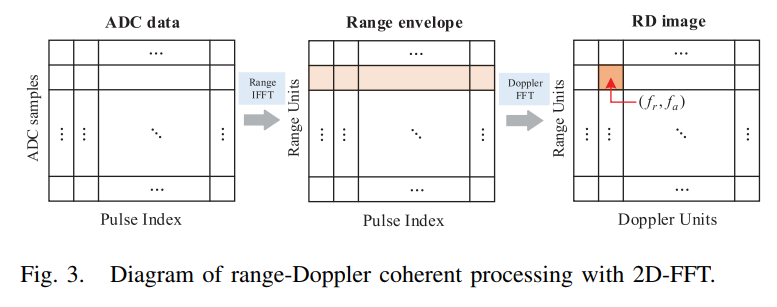
2.3 Basic Radar Signal Processing

• 1 Range FFT + Doppler FFT:

  • $\begin{array}{rl}& S_{IF}^{mn}\left(f_r,f_a\right)\\ & =G_m{G}_n\sum _{k=1}^K{\sigma }_k\cdot \exp \left(j{\psi }_k^{mn}\right)\cdot \exp \left(-j4\pi f_c\frac{R_{k0}}{c}\right)\\ & \cdot \mathrm{sinc}\left(T_p\left(f_r-2\mu \frac{R_k\left(n_a\right)}{c}\right)\right)\cdot \mathrm{sinc}\left(T_a\left(f_d-\frac{2f_c{v}_k}{c}\right)\right)\end{array}$
  • 

• 2 CFAR

• 3 DOA

• 4 坐标变换

  • $\left[\begin{array}{l}{\mathbf{x}}_{\mathbf{q}}\\ {\mathbf{y}}_{\mathbf{q}}\\ {\mathbf{z}}_{\mathbf{q}}\\ {\mathbf{v}}_{\mathbf{q}}\end{array}\right]=\left[\begin{array}{c}{R}_q\cdot \cos {\varphi }_q\cdot \cos {\theta }_q\\ R_q\cdot \cos {\varphi }_q\cdot \sin {\theta }_q\\ R_q\cdot \sin {\varphi }_q\\ f_d\cdot \lambda /2\end{array}\right],q=1,2,\dots ,Q$

3 High-Resolution PointClouds Imagery Generation

• focus on addressing above challenges:

  • 1 Optimal waveform orthogonality design
  • 2 High-dynamic high-resolution velocity measurement
  • 3 High-resolution DOA estimation

• 针对1和2：

  • a novel velocity ambiguity resolution algorithm combining with a TDM-DDM-MIMO framework

• 针对3:

  • a complex-valued deep convolution network (CV-DCN) of DOA-SR estimation

3.1 Proposed MIMO-Based Velocity Ambiguity Resolution Algorithm

• 仅使用 TDM 或者 DDM is almost unfeasible
• 需要设计一种方案 ： TDM-DDM-MIMO
  • 同时利用 TDM的inherent waveform orhogonality + DDM的high-dynamic high-resolution velocity measurement
  • 并且避免了DDM中的多目标检测问题 和 TDM的 PRF 与发射器数量之间的固有矛盾
• 同时，提出了一种基于 TDM-DDM-MIMO 的 dual-PRF waveforms velocity ambiguity resolution algorithm

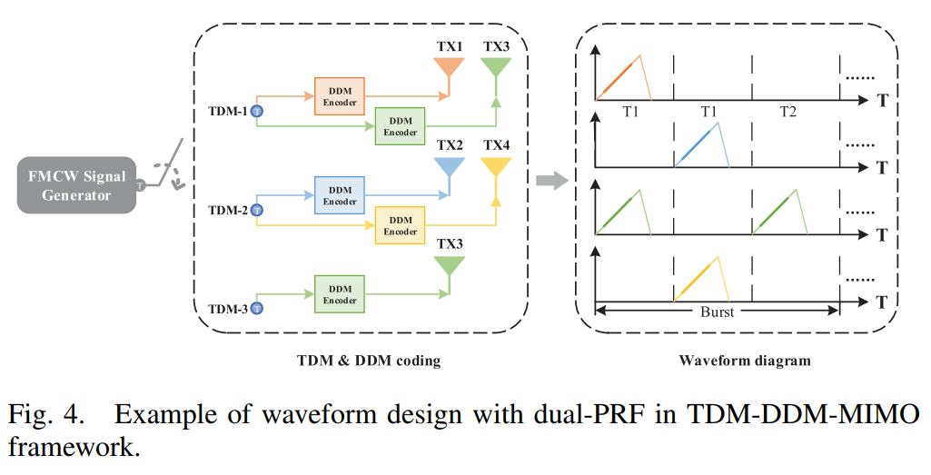
3.1.1 TDM-DDM-MIMO Framework

• TDM部分：
  • 三个均匀排列的发射机在三个相邻的传输周期内依次发射波形
• DDM部分：
  • 三个时分波形均产生两个不同的PRF
• 其余发射机：
  • 在前两个发射周期内合理分配，通过DDM编码发射正交波形
  • 在第三个发射周期内，仅保持一个发射机处于活动状态，其余发射机处于非活动状态 $\Rightarrow$ 避免了DDM中的多目标干扰问题
• 此外，对三个均匀放置的发射机的相应回波数据进行干涉相位处理，以提高明确的速度范围

下图是一个示例：

• T1: 表示 多天线传输（DDM编码）的前两个发射脉冲的PRI
• T2: 表示 单天线传输（DDM编码）的第三个发射脉冲的PRI

• For the same reveiver, the difference between the mixed phase difference ${\psi }_{1,2}$ and ${\psi }_{2,3}$ is:
  • $\Delta \psi ={\psi }_{2,3}-{\psi }_{1,2}=\frac{4\pi }{\lambda }v\left(T_2-T_1\right)+{ϵ}_{\Delta \psi }$
  • ${ϵ}_{\Delta \psi }$: the phase error deviating from the theoretical value $\Rightarrow$ can be ignored
• Due to $\Delta \psi \in [-\pi ,\pi ]$, the estimated unambiguous range of v is:
  • $v\in \left[-\frac{\lambda }{4\left(T_2-T_1\right)},\frac{\lambda }{4\left(T_2-T_1\right)}\right]$
• 相比于TDM-MIMO，TDM-DDM-MIMO的最大无歧义速度提高了：
  • $v_{\max }=\frac{MT1}{\left(T_2-T_1\right)}$ 倍

仿真实验

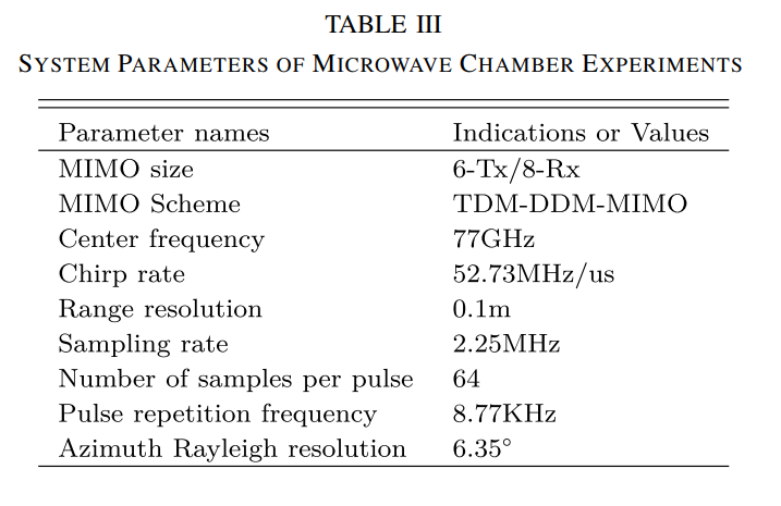
• 实验参数：

  

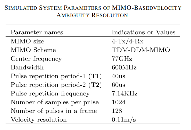
• 速度范围的提升：(compared with TDM)

  • original unambiguous velocity range: [-6.96m/s, 6.96m/s]
  • after the ambiguity resolution processing: [-48.70m/s, 48.70m/s]

• ghost目标的消除 (compared with DDM):

  • 
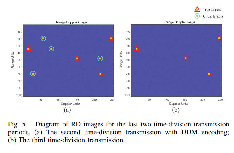
  • 最后一个单发射的T2: 没有ghost
  • T1(图a): 有ghost
  • 使用图b辅助图a

• 结论：

  • TDM-DDM-MIMO framework:
    • 1 保持了正交性
    • 2 提高了M倍的PRF
    • 3 避免了DDM中的多目标干扰问题

3.2 Proposed DL-Based DOA Estimation Algorithm

• traditional DOA algorithm的局限：
  • multi-snapshot data acquisition and high computational complexity
• 所提出的方法：DL-based super-resolution DOA algorithm
  • 1 spatial smoothing algorithm
  • 2 Deep learning technologies

(1) Pre-Processing of Single Snapshot Data (空间平滑算法)

• L-element ULA MIMO’s output:

  • $\begin{array}{rl}{X}_{azi}& ={\left[x_{az{i}_1},x_{az{i}_2},\dots ,x_{az{i}_L}\right]}^T\\ x_{az{i}_l}& =\sum _{q=1}^Q{x}_{r,q}\cdot \exp \left(j{\psi }_q^{az{i}_l}\right)+{ϵ}_{az{i}_l}\end{array}$
  • 其中，$\left[{\psi }_q^{az{i}_1},{\psi }_q^{az{i}_2},\dots ,{\psi }_q^{az{i}_L}\right]=[0,2\pi /\lambda \cdot d\sin \left({\theta }_q\right),\dots 2\pi /\lambda \cdot d(L-1)\sin \left({\theta }_q\right)]$： the array steering vector corresponding to ${\theta }_q$
  • d: baseline of the azimuth array

• 使用空间平滑算法的原因：

  • 空间谱估计算法通常利用多快拍数据构造协方差矩阵/spatial correlation matrix(然后通过特征分解来估计空间谱)
  • 但为了保证实时性，仅使用了单快拍数据
  • 因此，需要使用空间平滑算法 $\Rightarrow$ to equivalently construct the multi-snapshot data

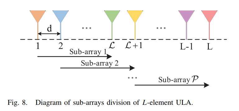
• Step1: 将 L 的线阵分为P个子阵列：

  • 

  • the array output of each sub-array ${\left[{\mathbf{x}}_1,{\mathbf{x}}_2,\dots ,{\mathbf{x}}_{\mathcal{P}}\right]}^T$:

    ✅ $\{\begin{array}{rl}{\mathbf{x}}_1=& \sum _{q=1}^Q{\mathbf{a}}_1\left({\theta }_q\right)\cdot x_{r,q}+{ϵ}_1\\ {\mathbf{x}}_2=& \sum _{q=1}^Q{\mathbf{a}}_2\left({\theta }_q\right)\cdot x_{r,q}+{ϵ}_2\\ & \dots \\ {\mathbf{x}}_{\mathcal{P}}=& \sum _{q=1}^Q{\mathbf{a}}_{\mathcal{P}}\left({\theta }_q\right)\cdot x_{r,q}+{ϵ}_{\mathcal{P}}\end{array}$

  • 其中，${\left[{\mathbf{a}}_1\left({\theta }_q\right),{\mathbf{a}}_2\left({\theta }_q\right),\dots ,{\mathbf{a}}_{\mathcal{P}}\left({\theta }_q\right)\right]}^T$： the steering vector of each sub-array corresponding to ${\theta }_q$

  • ${ϵ}_1,{ϵ}_2,\dots ,{ϵ}_{\mathcal{P}}$: the independent complex Gaussian white noise of each sub-array

• Step2: 逆向平滑，获得 the array output of each inverted sub-arrays:

  • ${\left[{\mathbf{x}}_{\mathcal{P}}^{\ast },{\mathbf{x}}_{\mathcal{P}-1}^{\ast },\dots ,{\mathbf{x}}_1^{\ast }\right]}^T$

• Step3: 合成multi-snapshot data $\tilde{\mathbf{x}}\left(t_n\right)$

  • 等价于：牺牲物理孔径来获得时间维度上的sampling
  • $\begin{array}{rl}\tilde{\mathbf{x}}\left(t_n\right)& ={\left[{\mathbf{x}}_1,{\mathbf{x}}_2,\dots ,{\mathbf{x}}_{\mathcal{P}},{\mathbf{x}}_{\mathcal{P}}^{\ast },\dots ,{\mathbf{x}}_1^{\ast }\right]}^T\\ & =\sum _{q=1}^Q\mathbf{a}\left({\theta }_q\right)\cdot x_{r,q}\left(t_n\right)+ϵ\left(t_n\right)\end{array}$
  • 其中， $\mathbf{a}\left({\theta }_q\right)$： the steering vector for sub-arrays with the same array manifold
  • $t_n=1,\dots ,2(L-\mathcal{L}+1)$: the index of snapshot

• Step4: 估计空间谱

  • then, the spatial correlation matrix of the adjusted multi-snapshot data can be estimated as: $\begin{array}{rl}\tilde{\mathbf{R}}& =\mathbb{E}\left[\tilde{\mathbf{x}}\left(t_n\right)\cdot {\tilde{\mathbf{x}}}^H\left(t_n\right)\right]\\ & =\sum _{q=1}^Q{\eta }_q\cdot \mathbf{a}\left({\theta }_q\right)\cdot {\mathbf{a}}^H\left({\theta }_q\right)+{\sigma }_{ϵ}^{2}I\end{array}$

  • 其中，${\eta }_q=\mathbb{E}\left[x_{r,q}\left(t_n\right)\cdot x_{r,q}^H\left(t_n\right)\right]$：the signal power on the direction of $q-th$ target

  • DOA估计：已知 correlation matrix $\tilde{\mathbf{R}}$，求${\eta }_q=\mathbb{E}\left[x_{r,q}\left(t_n\right)\cdot x_{r,q}^H\left(t_n\right)\right]$

  • $\tilde{\mathbf{R}}$的第$k$列可以rewritten 为：${\mathbf{r}}_{\kappa }=\tilde{\mathbf{R}}\cdot {\mathbf{e}}_{\kappa }\triangleq {\mathbf{A}}_{\kappa }\cdot \Gamma +{\sigma }_{ϵ}^2\cdot {\mathbf{e}}_{\kappa }$

    ✅ 其中，${\mathbf{A}}_{\kappa }=\left[\mathbf{a}\left({\theta }_1\right){\mathbf{a}}^H\left({\theta }_1\right){\mathbf{e}}_{\kappa },\dots ,\mathbf{a}\left({\theta }_Q\right){\mathbf{a}}^H\left({\theta }_Q\right){\mathbf{e}}_{\kappa }\right]$，${\mathbf{e}}_{\kappa }$：the $\kappa$-th column of the identity matrix (L × 1 vector with the κ-th element being “1” and others being “0”.)

  • 因此有：$\mathbf{r}=\left[{\mathbf{r}}_1;\cdots ;{\mathbf{r}}_{\mathcal{L}}\right]=\tilde{\mathbf{A}}\cdot \Gamma +{\sigma }_{ϵ}^2\Omega$

    ✅ 其中，$\tilde{\mathbf{A}}=\left[{\mathbf{A}}_1;\cdots ;{\mathbf{A}}_{\mathcal{L}}\right],\Omega =\left[{\tilde{\mathbf{e}}}_1;\cdots ;{\tilde{\mathbf{e}}}_{\mathcal{L}}\right]$.

  • 后续CV-DCN的任务：已知measurement vector $r$ 求 $\Gamma$ ，即：一个典型的逆问题

(2) CV-DCN Design

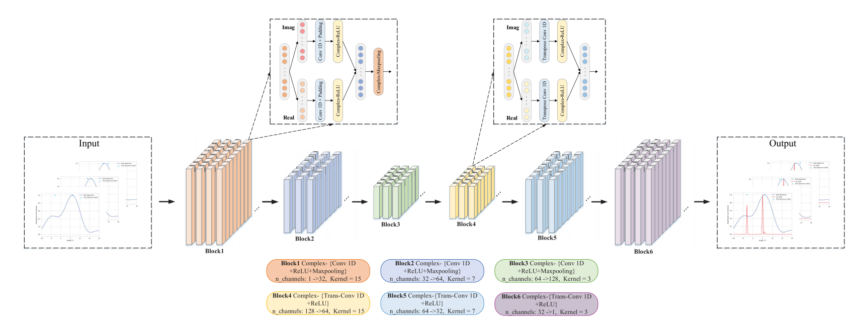
• 网络结构
  • 基于CNN + autoencoder
  • CV-DCN: has six blocks
• 1~3 blocks:
  • lower sampling processing
  • ComplexConv 1D + complex-valued ReLU + Complex max-pooling
• 4~6 blocks:
  • upper sampling processing
  • Complex-Trans-Conv 1D + complex-valued ReLU

• Complex Conv 1d:

  • 令$\mathbf{h}=x+jy$表示complex vector, $\mathbf{w}=a+jb$表示complex convolutional kernel
  • 则卷积过程表示为：$\left[\begin{array}{c}\mathcal{R}(\mathbf{w}\ast \mathbf{h})\\ \mathcal{I}(\mathbf{w}\ast \mathbf{h})\end{array}\right]=\left[\begin{array}{cc}a& -b\\ b& a\end{array}\right]\ast \left[\begin{array}{l}x\\ y\end{array}\right]$

• complex-valued ReLU (CReLU)

  • $C\mathrm{Re}LU(h)=\mathrm{ReLU}(\mathcal{R}(h))+j\mathrm{ReLU}(\mathcal{I}(h))$

• Complex max-pooling: 取maximum amplitude

• CV-DCN可以表示为：

  • ${\mathbf{o}}^{(n)}=\{\begin{array}{ll}\mathrm{CMP}\left(\mathrm{CReLU}\left({\mathbf{w}}^{(n)}\ast {\mathbf{x}}^{(n)}+{\mathcal{B}}^{(n)}\right)\right),& n=1,2,3.\\ \mathrm{CReLU}\left({\mathbf{w}}^{(n)}⊛{\mathbf{x}}^{(n)}+{\mathcal{B}}^{(n)}\right),& n=4,5,6.\end{array}$
  • 其中，${\mathbf{x}}^{(n)}$：the input of the $n$-th block; ${\mathbf{o}}^{(n)}$：the output of the $n$-th block;
  • ${\mathbf{w}}^{(n)}$：the convolutional kernel of the $n$-th block; ${\mathcal{B}}^{(n)}$：the bias of the $n$-th block;

(3) Learning Strategy

• 1st Stage: 数据集构建

  • 训练集：幅度和初始相位随机生成、空间平滑算法、合成回波
  • 验证集：生成与训练集保持相同规模、相同生成方式和相同数据分布的验证集

• 2st Stage: 训练

  • 损失函数：$\begin{array}{rl}\mathrm{LOSS}& =\mathbb{E}\left[\Vert \bar{\Theta }-\Theta {\Vert }_2+\beta \Vert \bar{\Theta }{\Vert }_1\right]\\ & =\frac{1}{\mathcal{N}}\sum _{n=1}^{\mathcal{N}}{\left({\bar{\Theta }}_n-{\Theta }_n\right)}^2+\beta \frac{1}{\mathcal{N}}\sum _{n=1}^{\mathcal{N}}\left|{\bar{\Theta }}_n\right|\end{array}$
  • 其中：${\Theta }_n$：the ground truth of the $n$-th training sample; ${\bar{\Theta }}_n$：predicted spectrum; $\mathcal{N}$: batchsize
  • 优化器：Adam, cosine learning rate
  • metric: $\mathrm{RMSE}(\bar{\theta },\theta )=\sqrt{\frac{1}{\mathcal{N}\mathcal{K}}{\sum }_{n=1}^{\mathcal{N}}{\sum }_{k=1}^{\mathcal{K}}{\left({\bar{\theta }}_k-{\theta }_k\right)}_n^2}$

4 Experimental Analysis

• 使用TI2243EVM模块和Pytorch框架,构建DL模型并训练

4.1 Super-Resolution DOA Estimation Experiments

A 仿真数据实验

• 构建大规模模拟数据集,并将-60°到60°的角范围划分为240个0.5°的网格

• 训练数据集630400个样本,验证集同规模;Epoch300,batch size100,学习率$10^{-}4$,权重衰减$10^{-}6$,$\beta =1.2\times 10^{-}3$

• 计算复杂度:CV-DCN 47.4Mflops,DCN 0.42Mflops;

• 性能评估:

  • 1. 比较CV-DCN和DCN,角分离2°到10°,SNR 10dB到20dB,CV-DCN表现更好,误差随SNR降低;
  • 2. 两个目标角度-40°到40°,恒定角分离3°,大多数CV-DCN误差<0.5°,DCN多失败;
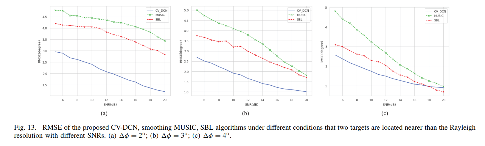
  • 3. 两个目标角分离小于分辨率6.35°,CV-DCN性能更稳定。

• 结果

  • 不同条件下DOA估计,CV-DCN匹配真值,误差主要<0.5°;DCN多失败。

  

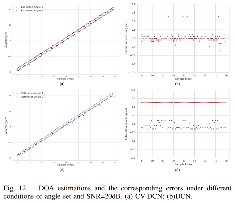
  • 实验参数

  

  • 不同算法在角分离2°到4°和SNR 5dB到20dB的RMSE,CV-DCN性能更稳定

  

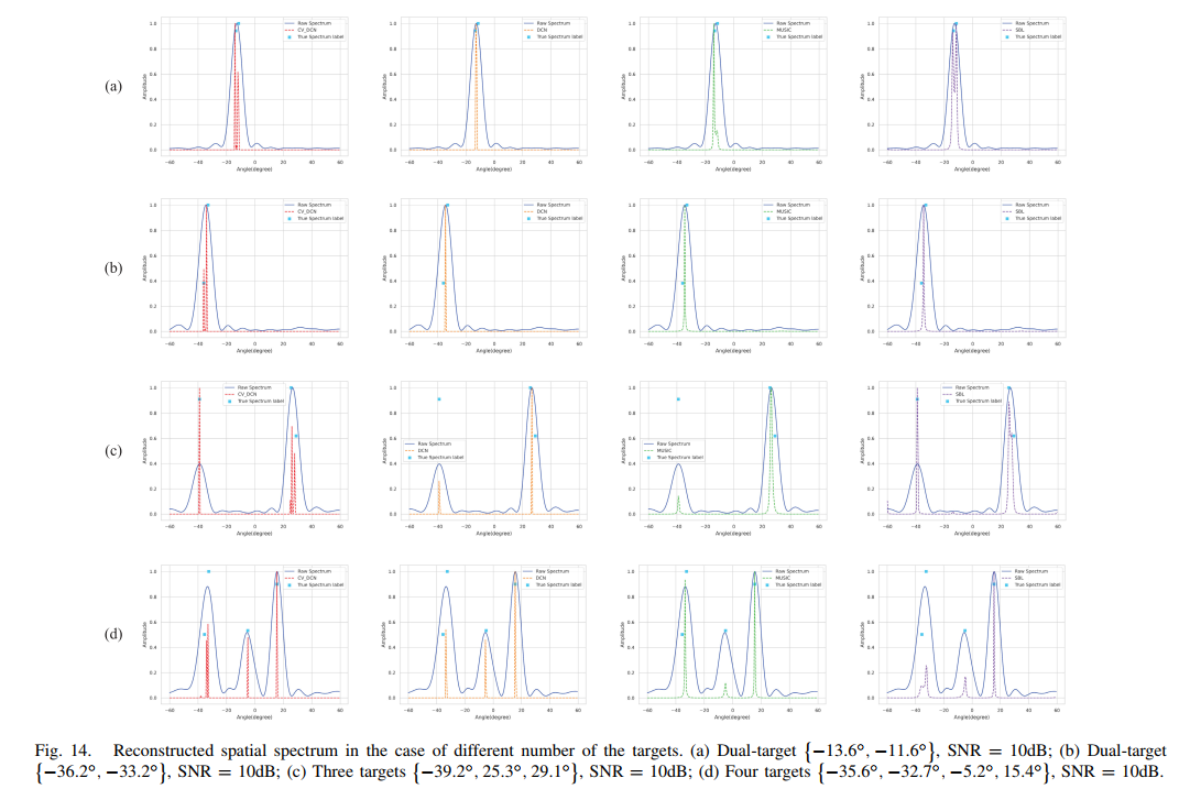
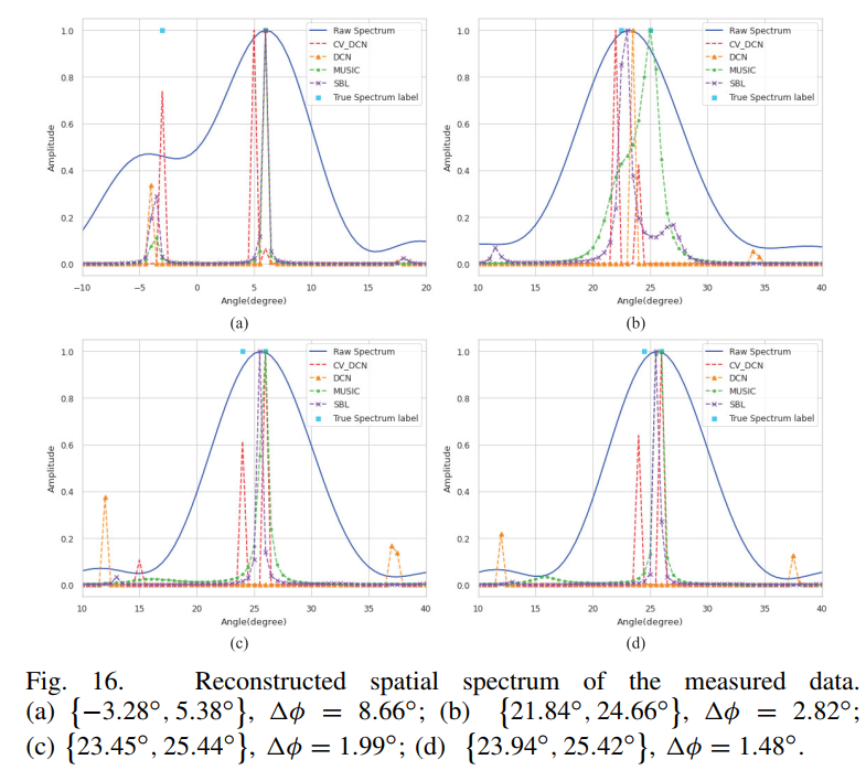
  • 原始谱,预测谱和理想标签,两目标和多目标情况,CV-DCN性能更好

  

B 实测数据实验

• 实验场景

  

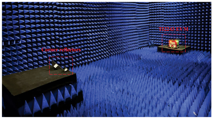
• results

  

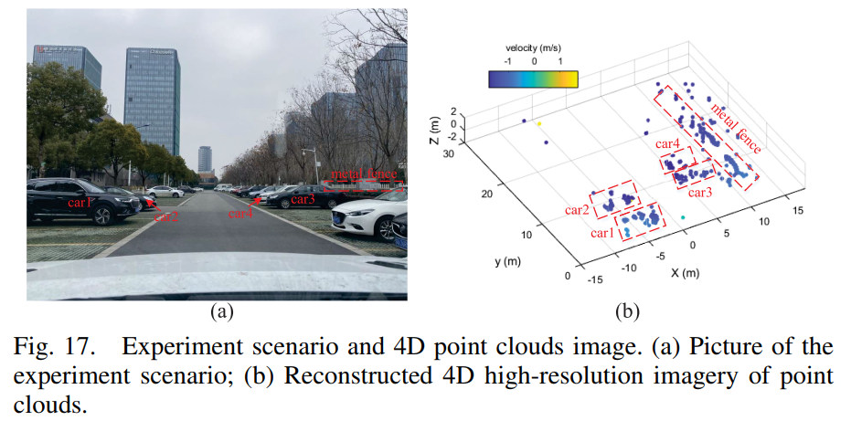
4.2 Extended to 4D Point Clouds Imaging

• 实验结果

  

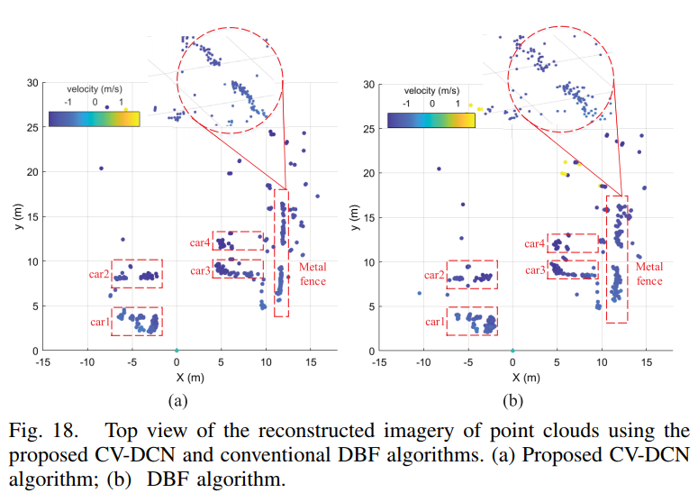
• 对比

5 Conclusion

• Novel algorithm of 4D high-resolution point clouds imagery
  • TDM-DDM-MIMO框架 $\Rightarrow$ 双PRF波形设计相结合,提出优秀速度误差分辨算法
  • 提出超分辨DOA估计算法,命名CV-DCN $\Rightarrow$ 利用神经网络的复值和自编码器结构,进一步利用空间谱的相位信息
• 实验
  • 超分辨DOA估计算法的有效性
  • 使用测量数据实验实现4D高分辨点云成像
• future work
  • 提升实际应用中的泛化能力