NNDL 作业9 RNN - SRN

简单循环网络（Simple Recurrent Network，SRN）只有一个隐藏层的神经网络．

目录

1. 实现SRN

（1）使用Numpy

（2）在1的基础上，增加激活函数tanh

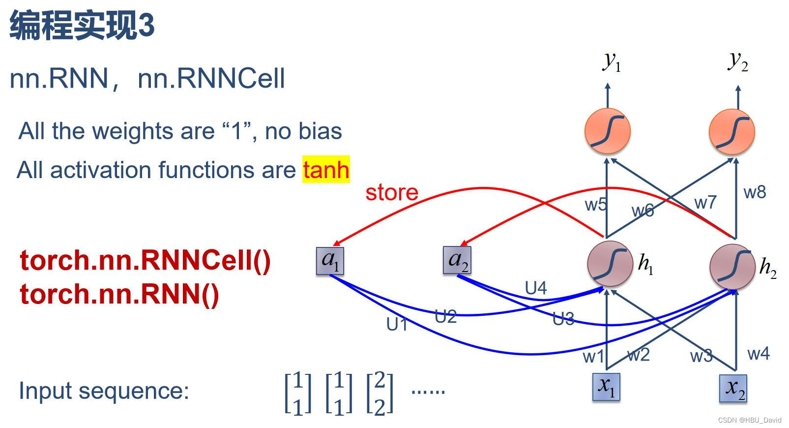
（3）使用nn.RNNCell实现

（4）使用nn.RNN实现

2. 实现“序列到序列”

3. “编码器-解码器”的简单实现

4.简单总结nn.RNNCell、nn.RNN

5.谈一谈对“序列”、“序列到序列”的理解

6.总结本周理论课和作业，写心得体会

---------------------------------------------------------------------------------------------------------------------------------

1. 实现SRN

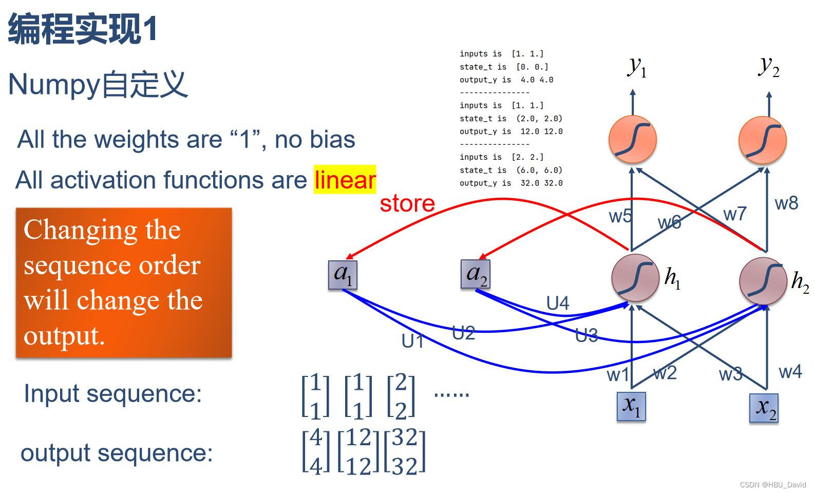
（1）使用Numpy

import numpy as np
 
inputs = np.array([[1., 1.],
                   [1., 1.],
                   [2., 2.]])  # 初始化输入序列
print('inputs is ', inputs)
 
state_t = np.zeros(2, )  # 初始化存储器
print('state_t is ', state_t)
 
w1, w2, w3, w4, w5, w6, w7, w8 = 1., 1., 1., 1., 1., 1., 1., 1.
U1, U2, U3, U4 = 1., 1., 1., 1.
print('--------------------------------------')
for input_t in inputs:
    print('inputs is ', input_t)
    print('state_t is ', state_t)
    in_h1 = np.dot([w1, w3], input_t) + np.dot([U2, U4], state_t)
    in_h2 = np.dot([w2, w4], input_t) + np.dot([U1, U3], state_t)
    state_t = in_h1, in_h2
    output_y1 = np.dot([w5, w7], [in_h1, in_h2])
    output_y2 = np.dot([w6, w8], [in_h1, in_h2])
    print('output_y is ', output_y1, output_y2)
    print('---------------')

结果：

调换顺序：

从实验看可以看出，对于循环神经网络来说，输入的顺序会影响训练结果。 

（2）在1的基础上，增加激活函数tanh

代码：

# 2. 在1的基础上，增加激活函数tanh
import numpy as np

print('在1的基础上，增加激活函数tanh :')
inputs = np.array([[1., 1.],
                   [1., 1.],
                   [2., 2.]])  # 初始化输入序列
print('inputs is ', inputs)

state_t = np.zeros(2, )  # 初始化存储器
print('state_t is ', state_t)

w1, w2, w3, w4, w5, w6, w7, w8 = 1., 1., 1., 1., 1., 1., 1., 1.
U1, U2, U3, U4 = 1., 1., 1., 1.
print('--------------------------------------')
for input_t in inputs:
    print('inputs is ', input_t)
    print('state_t is ', state_t)
    in_h1 = np.tanh(np.dot([w1, w3], input_t) + np.dot([U2, U4], state_t))
    in_h2 = np.tanh(np.dot([w2, w4], input_t) + np.dot([U1, U3], state_t))
    state_t = in_h1, in_h2
    output_y1 = np.dot([w5, w7], [in_h1, in_h2])
    output_y2 = np.dot([w6, w8], [in_h1, in_h2])
    print('output_y is ', output_y1, output_y2)
    print('---------------')

结果：

（3）使用nn.RNNCell实现

代码：

import torch
 
batch_size = 1
seq_len = 3  # 序列长度
input_size = 2  # 输入序列维度
hidden_size = 2  # 隐藏层维度
output_size = 2  # 输出层维度
 
# RNNCell
cell = torch.nn.RNNCell(input_size=input_size, hidden_size=hidden_size)
# 初始化参数 https://zhuanlan.zhihu.com/p/342012463
for name, param in cell.named_parameters():
    if name.startswith("weight"):
        torch.nn.init.ones_(param)
    else:
        torch.nn.init.zeros_(param)
# 线性层
liner = torch.nn.Linear(hidden_size, output_size)
liner.weight.data = torch.Tensor([[1, 1], [1, 1]])
liner.bias.data = torch.Tensor([0.0])
 
seq = torch.Tensor([[[1, 1]],
                    [[1, 1]],
                    [[2, 2]]])
hidden = torch.zeros(batch_size, hidden_size)
output = torch.zeros(batch_size, output_size)
 
for idx, input in enumerate(seq):
    print('=' * 20, idx, '=' * 20)
 
    print('Input :', input)
    print('hidden :', hidden)
 
    hidden = cell(input, hidden)
    output = liner(hidden)
    print('output :', output)

结果：

（4）使用nn.RNN实现

# 4. 使用nn.RNN实现
import torch
print('使用nn.RNN实现 :')
batch_size = 1
seq_len = 3
input_size = 2
hidden_size = 2
num_layers = 1
output_size = 2
 
cell = torch.nn.RNN(input_size=input_size, hidden_size=hidden_size, num_layers=num_layers)
for name, param in cell.named_parameters():  # 初始化参数
    if name.startswith("weight"):
        torch.nn.init.ones_(param)
    else:
        torch.nn.init.zeros_(param)
 
# 线性层
liner = torch.nn.Linear(hidden_size, output_size)
liner.weight.data = torch.Tensor([[1, 1], [1, 1]])
liner.bias.data = torch.Tensor([0.0])
 
inputs = torch.Tensor([[[1, 1]],
                       [[1, 1]],
                       [[2, 2]]])
hidden = torch.zeros(num_layers, batch_size, hidden_size)
out, hidden = cell(inputs, hidden)
 
print('Input :', inputs[0])
print('hidden:', 0, 0)
print('Output:', liner(out[0]))
print('--------------------------------------')
print('Input :', inputs[1])
print('hidden:', out[0])
print('Output:', liner(out[1]))
print('--------------------------------------')
print('Input :', inputs[2])
print('hidden:', out[1])
print('Output:', liner(out[2]))

结果：

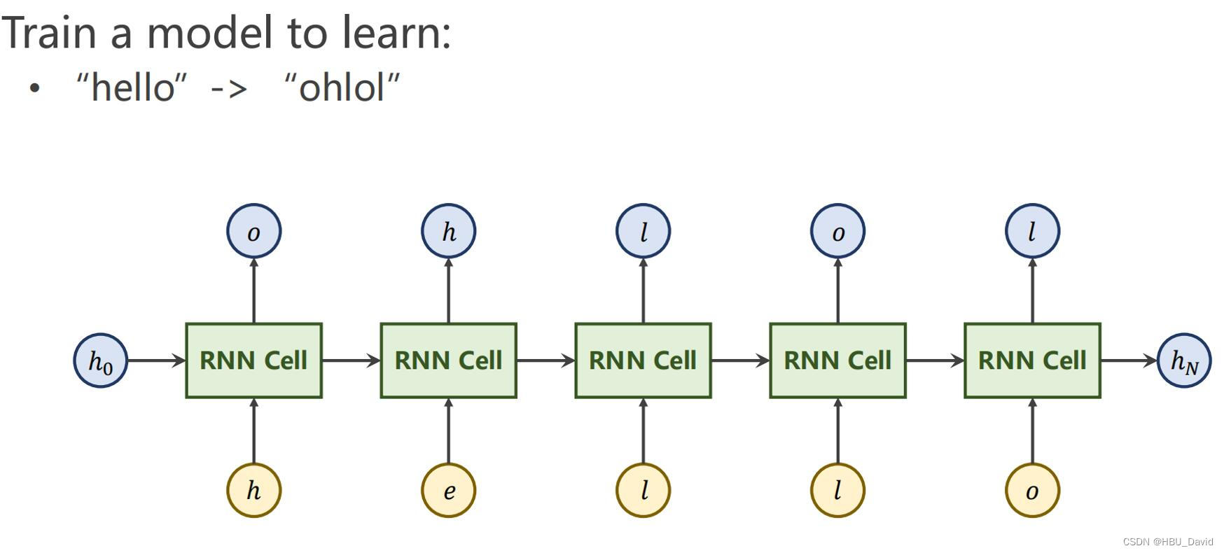
2. 实现“序列到序列”

观看视频，学习RNN原理，并实现视频P12中的教学案例

12.循环神经网络（基础篇）_哔哩哔哩_bilibili

 

（1）torch.RNNCell

seqLen:每个句子所含词的个数
batchSize：每次处理词的批数
InputSize：每个词嵌入向量的位数
dataset: (seq_size, batch_size, input_size)——>整个数据集维度
input: (batch_size, input_size)——>每个时间步处理的输入（input in dataset）
hidden: (batch_size, output_size)——>每次处理的隐层(即为output)

# RNNCell的使用
import torch

print('RNNCell的使用')
batch_size = 1
seq_len = 3
input_size = 4
hidden_size = 2

cell = torch.nn.RNNCell(input_size=input_size, hidden_size=hidden_size)

dataset = torch.randn(seq_len, batch_size, input_size)
hidden = torch.zeros(batch_size, hidden_size)

for idx, input in enumerate(dataset):
    print('=' * 20, idx, '=' * 20)
    print('input size:', input.shape)
    hidden = cell(input, hidden)
    print('outputs size:', hidden.shape)
    print(hidden)

输出结果：

（2）torch.RNN的使用

输入dataset：整个序列（seq_size, batch_size, input_size）   取每一个词input(batch_size, input_size)
隐层：(num_layers, batch_size, hidden_size)
输出（有两个）: output:h1~hn  (seq_size, batch_size, hidden_size)
              hidden: hn (num_layers, batch_size, hidden_size)

import torch
print('RNN的使用')
batch_size = 1
seq_len = 3
input_size = 4
hidden_size = 2
num_layers = 1
 
cell = torch.nn.RNN(input_size=input_size, hidden_size=hidden_size, num_layers=num_layers, batch_first=True)
 
inputs = torch.randn(batch_size, seq_len, input_size)
hidden = torch.zeros(num_layers, batch_size, hidden_size)
 
out, hidden = cell(inputs, hidden)
 
print('Output size:', out.shape)
print('Output:', out)
print('Hidden size:', hidden.shape)
print('Hidden:', hidden)

结果：

1.RNN与RNNCell相比多了一个num_layers，同时不用自己写循环
2.输出output是历史hidden记录， hidden为最后一个隐层输出
3.可以指定batch_first参数，使得以(batch_size, seq_len, input_size)进行输入  
（3）RNNCell的应用

import torch

print('基于RNNCell处理seq->seq任务')
# 1.参数设置
input_size = 4
hidden_size = 4  # 输出维度要与输入一致，才能在同一个表上查询
batch_size = 1

# 2.数据准备
index2char = ['e', 'h', 'l', 'o']  # 字典
x_data = [1, 0, 2, 2, 3]  # hello
y_data = [3, 1, 2, 3, 2]  # 标签：ohlol
# one-hot 查找表(维度为字典中词的个数)
one_hot_lookup = [[1, 0, 0, 0],  # 用来将x_data转换为one-hot向量的参照表
                  [0, 1, 0, 0],
                  [0, 0, 1, 0],
                  [0, 0, 0, 1]]
x_one_hot = [one_hot_lookup[x] for x in x_data]  # 转化为独热向量,维度(seq, batch, input)
dataset = torch.Tensor(x_one_hot).view(-1, batch_size,
                                       input_size)  # 转tensor后整理成(𝒔𝒆𝒒𝑳𝒆𝒏,𝒃𝒂𝒕𝒄𝒉𝑺𝒊𝒛𝒆,𝒊𝒏𝒑𝒖𝒕𝑺𝒊𝒛𝒆)
labels = torch.LongTensor(y_data).view(-1, 1)  # 每层对应一个类(seqLen,𝟏)计算交叉熵损失时标签不需要我们进行one-hot编码，其内部会自动进行处理


# 3.模型构建
class Model(torch.nn.Module):
    def __init__(self, input_size, hidden_size, batch_size):  # 需要指定输入，隐层，批
        super(Model, self).__init__()
        self.batch_size = batch_size
        self.input_size = input_size
        self.hidden_size = hidden_size
        self.rnncell = torch.nn.RNNCell(input_size=self.input_size, hidden_size=hidden_size)

    def forward(self, input, hidden):
        hidden = self.rnncell(input, hidden)
        return hidden

    def init_hidden(self):  # 只有在初始化隐藏层需要batch_size
        return torch.zeros(self.batch_size, self.hidden_size)


net = Model(input_size, hidden_size, batch_size)

# 4.损失和优化器
criterion = torch.nn.CrossEntropyLoss()
optimizer = torch.optim.Adam(net.parameters(), lr=0.1)

# 5.训练
for epoch in range(15):
    loss = 0
    optimizer.zero_grad()
    hidden = net.init_hidden()  # 初始化h0
    print('Predicted string:', end='')
    for input, label in zip(dataset, labels):
        hidden = net(input, hidden)
        loss += criterion(hidden, label)  # 这里要求总损失进行梯度下降（构建计算图），因此不能取item()
        _, idx = hidden.max(dim=1)  # 取出概率最大的索引
        print(index2char[idx.item()], end='')
    loss.backward()
    optimizer.step()
    print(',Epoch [%d / 15] loss:%.4f' % (epoch + 1, loss.item()))

结果：

对于输入序列进行独热编码，构建RNNCell，对每次输入的字符依次进入循环，进行训练。

（4）RNN的应用

import torch
print('基于RNN处理seq->seq任务')
# 1.参数设置
seq_len = 5
input_size = 4
hidden_size = 4
batch_size = 1
 
# 2.数据准备
index2char = ['e', 'h', 'l', 'o']
x_data = [1, 0, 2, 2, 3]
y_data = [3, 1, 2, 3, 2]
one_hot_lookup = [[1, 0, 0, 0],
                  [0, 1, 0, 0],
                  [0, 0, 1, 0],
                  [0, 0, 0, 1]]
x_one_hot = [one_hot_lookup[x] for x in x_data]
inputs = torch.Tensor(x_one_hot).view(-1, batch_size, input_size)
labels = torch.LongTensor(y_data)
 
# 3.模型构建
class Model(torch.nn.Module):
    def __init__(self, input_size, hidden_size, batch_size, num_layers=1):  # 需要指定输入，隐层，批
        super(Model, self).__init__()
        self.batch_size = batch_size
        self.input_size = input_size
        self.hidden_size = hidden_size
        self.num_layers = num_layers
        self.rnn = torch.nn.RNN(input_size=self.input_size, hidden_size=self.hidden_size, num_layers=self.num_layers)
 
    def forward(self, input):
        hidden = torch.zeros(self.num_layers,
                             self.batch_size,
                             self.hidden_size)
        out, _ = self.rnn(input, hidden)  # out: tensor of shape (seq_len, batch, hidden_size)
        return out.view(-1, self.hidden_size)  # 将输出的三维张量转换为二维张量,(𝒔𝒆𝒒𝑳𝒆𝒏×𝒃𝒂𝒕𝒄𝒉𝑺𝒊𝒛𝒆,𝒉𝒊𝒅𝒅𝒆𝒏𝑺𝒊𝒛𝒆)
 
 
net = Model(input_size, hidden_size, batch_size)
 
# 4.损失和优化器
criterion = torch.nn.CrossEntropyLoss()
optimizer = torch.optim.Adam(net.parameters(), lr=0.5)
 
# 5.训练
for epoch in range(15):
    optimizer.zero_grad()
    outputs = net(inputs)
    print(outputs.shape)
    loss = criterion(outputs, labels)
    loss.backward()
    optimizer.step()
 
    _, idx = outputs.max(dim=1)
    idx = idx.data.numpy()
    print('Predicted string: ', ''.join([index2char[x] for x in idx]), end='')
    print(',Epoch [%d / 15] loss:%.4f' % (epoch+1, loss.item()))

结果：

D:\anaconda\Anaconda\envs\pytorch\python.exe D:\pycharm\项目存放目录\main.py 
基于RNN处理seq->seq任务
torch.Size([5, 4])
Predicted string:  lhllh,Epoch [1 / 15] loss:1.3904
torch.Size([5, 4])
Predicted string:  ooloo,Epoch [2 / 15] loss:0.9733
torch.Size([5, 4])
Predicted string:  ohlol,Epoch [3 / 15] loss:0.7886
torch.Size([5, 4])
Predicted string:  ohlol,Epoch [4 / 15] loss:0.6133
torch.Size([5, 4])
Predicted string:  ohlol,Epoch [5 / 15] loss:0.5208
torch.Size([5, 4])
Predicted string:  ohlol,Epoch [6 / 15] loss:0.5252
torch.Size([5, 4])
Predicted string:  ohlol,Epoch [7 / 15] loss:0.4745
torch.Size([5, 4])
Predicted string:  ohlol,Epoch [8 / 15] loss:0.4684
torch.Size([5, 4])
Predicted string:  ohlol,Epoch [9 / 15] loss:0.4644
torch.Size([5, 4])
Predicted string:  ohlol,Epoch [10 / 15] loss:0.4554
torch.Size([5, 4])
Predicted string:  ohlol,Epoch [11 / 15] loss:0.4473
torch.Size([5, 4])
Predicted string:  ohlol,Epoch [12 / 15] loss:0.4428
torch.Size([5, 4])
Predicted string:  ohlol,Epoch [13 / 15] loss:0.4408
torch.Size([5, 4])
Predicted string:  ohlol,Epoch [14 / 15] loss:0.4398
torch.Size([5, 4])
Predicted string:  ohlol,Epoch [15 / 15] loss:0.4394

Process finished with exit code 0

从结果来看，损失比nn.RNNCell要低，但是预测结果到后来却开始错误了，‘ohlol’预测成了‘ohool’，可能是过拟合。 

输入：seq_size * batch_size * input_size
输出：seq_size * batch_size * hidden_size， 利用view变成（seq_size * batch_size, hidden_size）作为一个矩阵
labels: seq_size * batch_size * 1  (序列中每一个样本的分类)

最后的out和labels是针对整个seq进行比较计算损失的

使用的独热向量缺点：维度高、向量过于稀疏、是硬编码。

（5） 含嵌入层的RNN网络应用

在循环神经网络中，Embidding Layer用于将输入的离散型数据（如单词、字符等）转换为连续型的表示，以便于神经网络的处理。一文详解 Word2vec 之 Skip-Gram 模型（结构篇） | 雷峰网 (leiphone.com)

在之前的模型中，我们的输入被独热编码以后为一个稀疏矩阵，如果我们将一个1 x 10000的向量和10000 x 300的矩阵相乘，它会消耗相当大的计算资源，为了高效计算，在嵌入式的RNN网络中仅仅会选择矩阵中对应的向量中值为1的索引行（这个过程也被称为查表）。 
 

我们来看一下上图中的矩阵运算，左边分别是1 x 5和5 x 3的矩阵，结果应该是1 x 3的矩阵，按照矩阵乘法的规则，结果的第一行第一列元素为0 x 17 + 0 x 23 + 0 x 4 + 1 x 10 + 0 x 11 = 10，同理可得其余两个元素为12，19。如果10000个维度的矩阵采用这样的计算方式是十分低效的。

为了有效地进行计算，这种稀疏状态下不会进行矩阵乘法计算，可以看到矩阵的计算的结果实际上是矩阵对应的向量中值为1的索引，上面的例子中，左边向量中取值为1的对应维度为3（下标从0开始），那么计算结果就是矩阵的第3行（下标从0开始）—— [10, 12, 19]，这样模型中的隐层权重矩阵便成了一个”查找表“（lookup table），进行矩阵计算时，直接去查输入向量中取值为1的维度下对应的那些权重值。隐层的输出就是每个输入单词的“嵌入词向量”。

内容来自：一文详解 Word2vec 之 Skip-Gram 模型（结构篇） | 雷峰网 (leiphone.com)

import torch
print('含嵌入层的RNN网络')
# 1、确定参数
num_class = 4
input_size = 4
hidden_size = 8
embedding_size = 10
num_layers = 2
batch_size = 1
seq_len = 5
 
# 2、准备数据
index2char = ['e', 'h', 'l', 'o']  # 字典
x_data = [[1, 0, 2, 2, 3]]  # (batch_size, seq_len) 用字典中的索引（数字）表示来表示hello
y_data = [3, 1, 2, 3, 2]  # (batch_size * seq_len) 标签：ohlol
 
inputs = torch.LongTensor(x_data)  # (batch_size, seq_len)
labels = torch.LongTensor(y_data)  # (batch_size * seq_len)
 
 
# 3、构建模型
class Model(torch.nn.Module):
    def __init__(self):
        super(Model, self).__init__()
        self.emb = torch.nn.Embedding(num_class, embedding_size)
        self.rnn = torch.nn.RNN(input_size=embedding_size, hidden_size=hidden_size, num_layers=num_layers,
                                batch_first=True)
        self.fc = torch.nn.Linear(hidden_size, num_class)
 
    def forward(self, x):
        hidden = torch.zeros(num_layers, x.size(0), hidden_size)  # (num_layers, batch_size, hidden_size)
        x = self.emb(x)  # 返回(batch_size, seq_len, embedding_size)
        x, _ = self.rnn(x, hidden)  # 返回(batch_size, seq_len, hidden_size)
        x = self.fc(x)  # 返回(batch_size, seq_len, num_class)
        return x.view(-1, num_class)  # (batch_size * seq_len, num_class)
 
 
net = Model()
 
# 4、损失和优化器
criterion = torch.nn.CrossEntropyLoss()
optimizer = torch.optim.Adam(net.parameters(), lr=0.05)  # Adam优化器
 
# 5、训练
for epoch in range(15):
    optimizer.zero_grad()
    outputs = net(inputs)
    loss = criterion(outputs, labels)
    loss.backward()
    optimizer.step()
 
    _, idx = outputs.max(dim=1)
    idx = idx.data.numpy()
    print('Predicted string: ', ''.join([index2char[x] for x in idx]), end='')
    print(', Epoch [%d/15] loss: %.4f' % (epoch + 1, loss.item()))

3. “编码器-解码器”的简单实现

seq2seq的PyTorch实现_哔哩哔哩_bilibili

Seq2Seq的PyTorch实现 - mathor

# code by Tae Hwan Jung(Jeff Jung) @graykode, modify by wmathor
import torch
import numpy as np
import torch.nn as nn
import torch.utils.data as Data
 
device = torch.device('cuda' if torch.cuda.is_available() else 'cpu')
# S: Symbol that shows starting of decoding input
# E: Symbol that shows starting of decoding output
# ?: Symbol that will fill in blank sequence if current batch data size is short than n_step
 
letter = [c for c in 'SE?abcdefghijklmnopqrstuvwxyz']
letter2idx = {n: i for i, n in enumerate(letter)}
 
seq_data = [['man', 'women'], ['black', 'white'], ['king', 'queen'], ['girl', 'boy'], ['up', 'down'], ['high', 'low']]
 
# Seq2Seq Parameter
n_step = max([max(len(i), len(j)) for i, j in seq_data])  # max_len(=5)
n_hidden = 128
n_class = len(letter2idx)  # classfication problem
batch_size = 3
 
 
def make_data(seq_data):
    enc_input_all, dec_input_all, dec_output_all = [], [], []
 
    for seq in seq_data:
        for i in range(2):
            seq[i] = seq[i] + '?' * (n_step - len(seq[i]))  # 'man??', 'women'
 
        enc_input = [letter2idx[n] for n in (seq[0] + 'E')]  # ['m', 'a', 'n', '?', '?', 'E']
        dec_input = [letter2idx[n] for n in ('S' + seq[1])]  # ['S', 'w', 'o', 'm', 'e', 'n']
        dec_output = [letter2idx[n] for n in (seq[1] + 'E')]  # ['w', 'o', 'm', 'e', 'n', 'E']
 
        enc_input_all.append(np.eye(n_class)[enc_input])
        dec_input_all.append(np.eye(n_class)[dec_input])
        dec_output_all.append(dec_output)  # not one-hot
 
    # make tensor
    return torch.Tensor(enc_input_all), torch.Tensor(dec_input_all), torch.LongTensor(dec_output_all)
 
 
'''
enc_input_all: [6, n_step+1 (because of 'E'), n_class]
dec_input_all: [6, n_step+1 (because of 'S'), n_class]
dec_output_all: [6, n_step+1 (because of 'E')]
'''
enc_input_all, dec_input_all, dec_output_all = make_data(seq_data)
 
 
class TranslateDataSet(Data.Dataset):
    def __init__(self, enc_input_all, dec_input_all, dec_output_all):
        self.enc_input_all = enc_input_all
        self.dec_input_all = dec_input_all
        self.dec_output_all = dec_output_all
 
    def __len__(self):  # return dataset size
        return len(self.enc_input_all)
 
    def __getitem__(self, idx):
        return self.enc_input_all[idx], self.dec_input_all[idx], self.dec_output_all[idx]
 
 
loader = Data.DataLoader(TranslateDataSet(enc_input_all, dec_input_all, dec_output_all), batch_size, True)
 
 
# Model
class Seq2Seq(nn.Module):
    def __init__(self):
        super(Seq2Seq, self).__init__()
        self.encoder = nn.RNN(input_size=n_class, hidden_size=n_hidden, dropout=0.5)  # encoder
        self.decoder = nn.RNN(input_size=n_class, hidden_size=n_hidden, dropout=0.5)  # decoder
        self.fc = nn.Linear(n_hidden, n_class)
 
    def forward(self, enc_input, enc_hidden, dec_input):
        # enc_input(=input_batch): [batch_size, n_step+1, n_class]
        # dec_inpu(=output_batch): [batch_size, n_step+1, n_class]
        enc_input = enc_input.transpose(0, 1)  # enc_input: [n_step+1, batch_size, n_class]
        dec_input = dec_input.transpose(0, 1)  # dec_input: [n_step+1, batch_size, n_class]
 
        # h_t : [num_layers(=1) * num_directions(=1), batch_size, n_hidden]
        _, h_t = self.encoder(enc_input, enc_hidden)
        # outputs : [n_step+1, batch_size, num_directions(=1) * n_hidden(=128)]
        outputs, _ = self.decoder(dec_input, h_t)
 
        model = self.fc(outputs)  # model : [n_step+1, batch_size, n_class]
        return model
 
 
model = Seq2Seq().to(device)
criterion = nn.CrossEntropyLoss().to(device)
optimizer = torch.optim.Adam(model.parameters(), lr=0.001)
 
for epoch in range(5000):
    for enc_input_batch, dec_input_batch, dec_output_batch in loader:
        # make hidden shape [num_layers * num_directions, batch_size, n_hidden]
        h_0 = torch.zeros(1, batch_size, n_hidden).to(device)
 
        (enc_input_batch, dec_intput_batch, dec_output_batch) = (
        enc_input_batch.to(device), dec_input_batch.to(device), dec_output_batch.to(device))
        # enc_input_batch : [batch_size, n_step+1, n_class]
        # dec_intput_batch : [batch_size, n_step+1, n_class]
        # dec_output_batch : [batch_size, n_step+1], not one-hot
        pred = model(enc_input_batch, h_0, dec_intput_batch)
        # pred : [n_step+1, batch_size, n_class]
        pred = pred.transpose(0, 1)  # [batch_size, n_step+1(=6), n_class]
        loss = 0
        for i in range(len(dec_output_batch)):
            # pred[i] : [n_step+1, n_class]
            # dec_output_batch[i] : [n_step+1]
            loss += criterion(pred[i], dec_output_batch[i])
        if (epoch + 1) % 1000 == 0:
            print('Epoch:', '%04d' % (epoch + 1), 'cost =', '{:.6f}'.format(loss))
 
        optimizer.zero_grad()
        loss.backward()
        optimizer.step()
 
 
# Test
def translate(word):
    enc_input, dec_input, _ = make_data([[word, '?' * n_step]])
    enc_input, dec_input = enc_input.to(device), dec_input.to(device)
    # make hidden shape [num_layers * num_directions, batch_size, n_hidden]
    hidden = torch.zeros(1, 1, n_hidden).to(device)
    output = model(enc_input, hidden, dec_input)
    # output : [n_step+1, batch_size, n_class]
 
    predict = output.data.max(2, keepdim=True)[1]  # select n_class dimension
    decoded = [letter[i] for i in predict]
    translated = ''.join(decoded[:decoded.index('E')])
 
    return translated.replace('?', '')
 
 
print('test')
print('man ->', translate('man'))
print('mans ->', translate('mans'))
print('king ->', translate('king'))
print('black ->', translate('black'))
print('up ->', translate('up'))

结果:

4.简单总结nn.RNNCell、nn.RNN

nn.RNNCell：

nn.RNNCell是PyTorch中的一个类，用于定义一个RNN单元的计算逻辑。它接受一个输入和一个隐藏状态，并输出一个新的隐藏状态。

在每个时间步上，RNNCell使用相同的权重对输入和隐藏状态进行计算。nn.RNN是一个多层的RNN模型，它由多个RNNCell组成，可以进行序列数据的处理。

• RNNCell的结构：

nn.RNN:

nn.RNN将每个时间步的输入和前一个时间步的隐藏状态作为RNNCell的输入，并产生当前时间步的输出和隐藏状态。

nn.RNN可以根据需要设置层数、隐藏状态的维度、激活函数等参数来构建不同规模和功能的RNN模型。

• 若干RNN Cell组成RNN：

图片来源：【23-24 秋学期】NNDL 作业9 RNN - SRN-CSDN博客

总结：

nn.RNNCell和nn.RNN在实现上有一些区别。

nn.RNNCell是一个单独的RNN单元，它只能处理一个时间步的输入，并输出一个隐藏状态。而nn.RNN是由多个RNNCell组成的多层RNN模型，它可以处理整个序列，并且可以输出整个序列的隐藏状态。因此，nn.RNN比nn.RNNCell更适合处理序列数据。

此外，nn.RNNCell需要手动编写循环结构来处理整个序列数据，而nn.RNN会自动处理序列数据的循环结构，因此在使用上nn.RNN更加方便。

另外，nn.RNN可以设置bidirectional参数来构建双向RNN模型，而nn.RNNCell无法实现双向RNN。

总的来说，nn.RNNCell是 nn.RNN 的基本组成单元，nn.RNN是对多个 nn.RNNCell 的封装，提供了更高层次的序列处理功能和便捷性。

5.谈一谈对“序列”、“序列到序列”的理解

序列是指一系列按照顺序排列的数据，比如语音信号、时间序列数据、自然语言句子等。序列数据的特点是具有时序关系，每个数据点的意义往往依赖于其前面或后面的数据。

序列到序列（Sequence-to-Sequence，简称Seq2Seq）是一种常见的模型架构，主要用于将一个序列作为输入，经过模型处理后生成另一个序列作为输出。Seq2Seq模型常用于机器翻译、文本摘要、对话生成等任务。

Seq2Seq模型通常由编码器（Encoder）和解码器（Decoder）组成。编码器将输入序列转化为一个固定维度的向量，这个向量通常被称为上下文向量或隐藏状态，它包含了输入序列的信息。解码器根据上下文向量来生成输出序列，每个时间步产生一个输出。

6.总结本周理论课和作业，写心得体会

1. 循环神经网络（Recurrent Neural Network，RNN）通过对当前时间步的输入和前一个时间步的隐藏状态进行计算，每次计算都会使用上次计算的结果和本次的输入来计算，计算的结果一部分用于输出一部分被保存用于下次循环输入。

2. nn.RNNCell是PyTorch中的一个类，用于定义一个RNN单元的计算逻辑，只能处理一个时间步的输入，并输出一个隐藏状态。nn.RNN是由多个RNNCell组成的多层RNN模型，可以处理整个序列，并输出整个序列的隐藏状态。

3. RNN的应用广泛，常见的包括：

   • 序列分类：将一个序列作为输入，通过RNN模型进行分类预测
   • 序列生成：通过RNN模型根据前面的输入序列生成一个新的序列

4. 序列到分类（Sequence-to-Classification）是将一个序列作为输入，通过RNN模型预测它所属的类别。

5. 序列到序列（Sequence-to-Sequence）是将一个序列作为输入，通过RNN模型生成另一个序列作为输出。

6. 经过这一周的学习，最大的理解就是循环神经网络，通过是实验课和理论课的结合，真正明白了循环神经网络的原理，明白了自己的代码出错的原因，虽然依旧有的时候不能完全融会贯通，但是这周的课程对我的帮助依然很大。