UPGMA算法树的hierarchy回归

最新推荐文章于 2024-08-08 19:26:43 发布

绝对不要看眼睛里的郁金香

最新推荐文章于 2024-08-08 19:26:43 发布

阅读量4.9k

点赞数

UPGMA (Unweighted Pair Group Method with Arithmetic Mean) is a simple agglomerative (bottom-up) hierarchical clustering method. The method is generally attributed to Sokal and Michener.^[1]

The UPGMA method is similar to its weighted variant, the WPGMA method.

Algorithm

The UPGMA algorithm constructs a rooted tree (dendrogram) that reflects the structure present in a pairwise similarity matrix (or a dissimilarity matrix). At each step, the nearest two clusters are combined into a higher-level cluster. The distance between any two clusters A and B, each of size (i.e., cardinality) ${|\mathcal{A}|}$ and ${|\mathcal{B}|}$ , is taken to be the average of all distances $d(x,y)$ between pairs of objects $x$ in $\mathcal{A}$ and $y$ in $\mathcal{B}$ , that is, the mean distance between elements of each cluster:

{1 \over {|\mathcal{A}|\cdot|\mathcal{B}|}}\sum_{x \in \mathcal{A}}\sum_{ y \in \mathcal{B}} d(x,y)

In other words, at each clustering step, the updated distance between the joined clusters $\mathcal{A} \cup \mathcal{B}$ and a new cluster $X$ is given by the proportional averaging of the $d_{\mathcal{A},X}$ and $d_{\mathcal{B},X}$ distances:

$d_{(\mathcal{A} \cup \mathcal{B}),X} = \frac{|\mathcal{A}| \cdot d_{\mathcal{A},X} + |\mathcal{B}| \cdot d_{\mathcal{B},X}}{|\mathcal{A}| + |\mathcal{B}|}$

The UPGMA algorithm produces rooted dendrograms and requires a constant-rate assumption - that is, it assumes an ultrametric tree in which the distances from the root to every branch tip are equal. When the tips are molecular data (i.e., DNA, RNA and protein), the ultrametricity assumption is called the molecular clock.

Working example

First step

First clustering

Let us assume that we have five elements $(a,b,c,d,e)$ and the following matrix $D_1$ of pairwise distances between them :

	a	b	c	d	e
a	0	17	21	31	23
b	17	0	30	34	21
c	21	30	0	28	39
d	31	34	28	0	43
e	23	21	39	43	0

In this example, 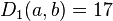$D_1 (a,b)=17$ is the smallest value of $D_1$ , so we join elements $a$ and $b$ .

First branch length estimation

Let $u$ denote the node to which $a$ and $b$ are now connected. Setting $\delta(a,u)=\delta(b,u)=D_1(a,b)/2$ ensures that elements $a$ and $b$ are equidistant from $u$ . This corresponds to the expectation of the ultrametricity hypothesis. The branches joining $a$ and $b$ to $u$ then have lengths $\delta(a,u)=\delta(b,u)=17/2=8.5$ (see the final dendrogram)

First distance matrix update

We then proceed to update the initial distance matrix $D_1$ into a new distance matrix $D_2$ (see below), reduced in size by one row and one column because of the clustering of $a$ with $b$ . Bold values in $D_2$ correspond to the new distances, calculated by averaging distances between the first cluster $(a,b)$ and each of the remaining elements:

$D_2((a,b),c)=(D_1(a,c) \times 1 + D_1(b,c) \times 1)/(1+1)=(21+30)/2=25.5$

$D_2((a,b),d)=(D_1(a,d) + D_1(b,d))/2=(31+34)/2=32.5$

$D_2((a,b),e)=(D_1(a,e) + D_1(b,e))/2=(23+21)/2=22$

Italicized values in $D_2$ are not affected by the matrix update as they correspond to distances between elements not involved in the first cluster.

Second step

Second clustering

We now reiterate the three previous steps, starting from the new distance matrix $D_2$

	(a,b)	c	d	e
(a,b)	0	25.5	32.5	22
c	25.5	0	28	39
d	32.5	28	0	43
e	22	39	43	0

Here, $D_2 ((a,b),e)=22$ is the smallest value of $D_2$ , so we join cluster $(a,b)$ and element $e$ .

Second branch length estimation

Let $v$ denote the node to which $(a,b)$ and $e$ are now connected. Because of the ultrametricity constraint, the branches joining $a$ or $b$ to $v$ , and $e$ to $v$ are equal and have the following length: $\delta(a,v)=\delta(b,v)=\delta(e,v)=22/2=11$

We deduce the missing branch length: $\delta(u,v)=\delta(e,v)-\delta(a,u)=\delta(e,v)-\delta(b,u)=11-8.5=2.5$ (see the final dendrogram)

Second distance matrix update

We then proceed to update $D_2$ into a new distance matrix $D_3$ (see below), reduced in size by one row and one column because of the clustering of $(a,b)$ with $e$ . Bold values in $D_3$ correspond to the new distances, calculated by proportional averaging:

$D_3(((a,b),e),c)=(D_2((a,b),c) \times 2 + D_2(e,c) \times 1)/(2+1)=(25.5 \times 2 + 39 \times 1)/3=30$

Thanks to this proportional average, the calculation of this new distance accounts for the larger size of the $(a,b)$ cluster (two elements) with respect to $e$ (one element). Similarly:

$D_3(((a,b),e),d)=(D_2((a,b),d) \times 2 + D_2(e,d) \times 1)/(2+1)=(32.5 \times 2 + 43 \times 1)/3=36$

Proportional averaging therefore gives equal weight to the initial distances of matrix $D_1$ . This is the reason why the method is unweighted, not with respect to the mathematical procedure but with respect to the initial distances.

Third step

Third clustering

We again reiterate the three previous steps, starting from the updated distance matrix $D_3$ .

	((a,b),e)	c	d
((a,b),e)	0	30	36
c	30	0	28
d	36	28	0

Here, $D_3 (c,d)=28$ is the smallest value of $D_3$ , so we join elements $c$ and $d$ .

Third branch length estimation

Let $w$ denote the node to which $c$ and $d$ are now connected. The branches joining $c$ and $d$ to $w$ then have lengths $\delta(c,w)=\delta(d,w)=28/2=14$ (see the final dendrogram)

Third distance matrix update

There is a single entry to update, keeping in mind that the two elements $c$ and $d$ each have a contribution of $1$ in the average computation:

$D_4((c,d),((a,b),e))=(D_3(c,((a,b),e)) \times 1 + D_3(d,((a,b),e)) \times 1)/(1+1)=(30 \times 1 + 36 \times 1)/2=33$

Final step

The final $D_4$ matrix is:

	((a,b),e)	(c,d)
((a,b),e)	0	33
(c,d)	33	0

So we join clusters $((a,b),e)$ and $(c,d)$ .

Let $r$ denote the (root) node to which $((a,b),e)$ and $(c,d)$ are now connected. The branches joining $((a,b),e)$ and $(c,d)$ to $r$ then have lengths:

$\delta(((a,b),e),r)=\delta((c,d),r)=33/2=16.5$

We deduce the two remaining branch lengths:

$\delta(v,r)=\delta(((a,b),e),r)-\delta(e,v)=16.5-11=5.5$

$\delta(w,r)=\delta((c,d),r)-\delta(c,w)=16.5-14=2.5$

The UPGMA dendrogram

The dendrogram is now complete. It is ultrametric because all tips ( $a$ to $e$ ) are equidistant from $r$ :

$\delta(a,r)=\delta(b,r)=\delta(e,r)=\delta(c,r)=\delta(d,r)=16.5$

The dendrogram is therefore rooted by $r$ , its deepest node.

Uses

In ecology, it is one of the most popular methods for the classification of sampling units (such as vegetation plots) on the basis of their pairwise similarities in relevant descriptor variables (such as species composition).^[2]
In bioinformatics, UPGMA is used for the creation of phenetic trees (phenograms). UPGMA was initially designed for use in protein electrophoresis studies, but is currently most often used to produce guide trees for more sophisticated algorithms. This algorithm is for example used in sequence alignment procedures, as it proposes one order in which the sequences will be aligned. Indeed, the guide tree aims at grouping the most similar sequences, regardless of their evolutionary rate or phylogenetic affinities, and that is exactly the goal of UPGMA.^[3]
In phylogenetics, UPGMA assumes a constant rate of evolution (molecular clock hypothesis), and is not a well-regarded method for inferring relationships unless this assumption has been tested and justified for the data set being used.

Time complexity

A trivial implementation of the algorithm to construct the UPGMA tree has $O(n^3)$ time complexity, and using a heap for each cluster to keep its distances from other cluster reduces its time to $O(n^2 \log n)$ . Fionn Murtagh presented some other approaches for special cases, a $O(k3^kn^2)$ time algorithm by Day and Edelsbrunner^[4] for k-dimensional data that is optimal $O(n^2)$ for constant k, and another $O(n^2)$ algorithm for restricted inputs, when "the anglomerative strategy satisfies the reducibility property."^[5]