【概率方法】MCMC 之 Gibbs 采样

上一篇文章讲到，MCMC 中的 HM 算法，它可以解决拒绝采样效率低的问题，但是实际上，当维度高的时候 HM 算法还是在同时处理多个维度，以两个变量 $\mathbf{x}=[x,y]$ 来说，也就是同时从联合分布里面 $p(\mathbf{x})=p(x,y)$ 进行采样，在某些情况下有维度灾难的问题。

有些时候，我们从联合分布 $p(x,y)$ 里面采样很难，但是从条件分布 $p(x|y),p(y|x)$ 里面采样很容易，

Gibbs 采样

为了解决维度灾难的问题，Gibbs 把直接从联合分布$p(x,y)$里面进行采样的问题转化成了逐个对每一个维度的条件分布进行采样 ：
对于二维情况，我们先得到每一个维度在给定其他维度时候的条件分布：
$$p(x|y),p(y|x)$$
先从一个任意选择的点$(x_0,y_0)$ 开始。
先给定$y_0$ ，采样 $x_1$：$$p(x_1|y_0)$$
再给定$x_1$，采样 $y_1$：$$p(y_1|x_1)$$

对所有维度轮换采样完成之后，就得到了新的采样点$(x_1,y_1)$，如此进行下去，采样得到整个序列
{ x 0 , . . . , x t } = { ( x 0 , y 0 ) , . . . , ( x t , y t ) } \{\mathbf{x}_0,...,\mathbf{x}_t\} = \{(x_0,y_0),...,(x_t,y_t)\} {x0​,...,xt​}={(x0​,y0​),...,(xt​,yt​)}

优点

• Gibbs 采样接受率为 1，采样效率更高
• 在知道各个维度的条件分布的时候，可以处理高维分布

坑

• 由于马尔可夫性，前后的样本是相关的，所以也可以用 Thinning 降低自相关性，或者其他方法。
• 当目标分布比较极端的时候可能难以收敛
• 

代码

import numpy as np
import matplotlib.pyplot as plt
from scipy.stats import pearsonr

# Goal: Sample from bivariate Normal

automatic_samples = np.random.multivariate_normal([0,0], [[1, 0.5], [0.5,1]], 10000)
plt.scatter(automatic_samples[:,0], automatic_samples[:,1], s=5)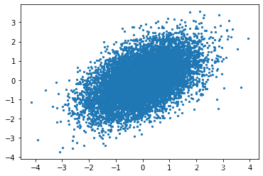![请添加图片描述](https://img-blog.csdnimg.cn/direct/b7f96ec7214f4c64be016e1a20df48f6.png)

# Gibbs Sampling

samples = {'x': [1], 'y': [-1]}

num_samples = 10000

for _ in range(num_samples):
    curr_y = samples['y'][-1]
    new_x = np.random.normal(curr_y/2, np.sqrt(3/4))
    new_y = np.random.normal(new_x/2, np.sqrt(3/4))
    samples['x'].append(new_x)
    samples['y'].append(new_y)

plt.scatter(samples['x'], samples['y'], s=5)

和 numpy 自带采样的分布是匹配的

plt.hist(automatic_samples[:,0], bins=20, density=True, alpha=0.5)
plt.hist(samples['x'], bins=20, density=True, alpha=0.5)

plt.hist(automatic_samples[:,1], bins=20, density=True, alpha=0.5)
plt.hist(samples['y'], bins=20, density=True, alpha=0.5)

查看相关性

plt.scatter(automatic_samples[:-1,0], automatic_samples[1:,0], s=5)
print(pearsonr(automatic_samples[:-1,0], automatic_samples[1:,0])[0])

plt.scatter(samples['x'][:-1], samples['x'][1:], s=5)
print(pearsonr(samples['x'][:-1], samples['x'][1:])[0])