


最近我们被客户要求撰写关于随机波动率SV模型可视化的研究报告,包括一些图形和统计输出。
相关视频:
随机波动率SV模型原理和Python对标普SP500股票指数时间序列波动性预测
相关视频:马尔可夫链原理可视化解释与R语言区制转换Markov regime switching实例
马尔可夫链原理可视化解释与R语言区制转换Markov regime switching实例
,时长07:25
相关视频
马尔可夫链蒙特卡罗方法MCMC原理与R语言实现
,时长08:47
在这个例子中,我们考虑马尔可夫转换随机波动率模型。
统计模型
让  是因变量和
是因变量和  未观察到的对数波动率 . 随机波动率模型定义如下

区制变量  遵循具有转移概率的二态马尔可夫过程

 表示均值的正态分布
  和方差
和方差  .
.
BUGS语言统计模型
文件“ssv.bug”的内容:
file = 'ssv.bug'; % BUGS模型文件名

model
{
  x[1] ~ dnorm(mm[1], 1/sig^2)
  y[1] ~ dnorm(0, exp(-x[1]))

  for (t in 2:tmax)
  {
    c[t] ~ dcat(ifelse(c[t-1]==1, pi[1,], pi[2,]))
    mm[t] <- alp[1] * (c[t]==1) + alp[2]*(c[t]==2) + ph*x[t-1]
安装
- 下载Matlab最新版本
- 将存档解压缩到某个文件夹中
- 将程序文件夹添加到 Matlab 搜索路径
addpath(path)通用设置
lightblue
lightred

% 设置随机数生成器的种子以实现可重复性
if eLan 'matlab', '7.2')
    rnd('state', 0)
else
    rng('default')
end
加载模型和数据
模型参数
tmax = 100;
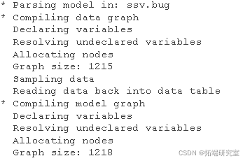
sig = .4;解析编译BUGS模型,以及样本数据
model(file, data, 'sample', true);
data = model;
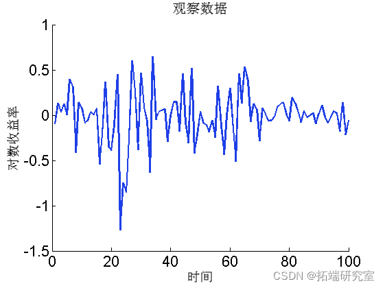
绘制数据
figure('nae', 'Lrtrs')
plot(1:tmax, dt.y)
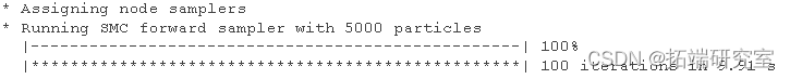
Biips 序列蒙特卡罗SMC
运行SMC
n_part = 5000; % 粒子数
  {'x'}; % 要监控的变量
 smc =  samples(npart);
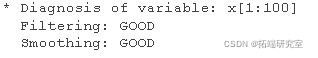
算法的诊断。
diag (smc);
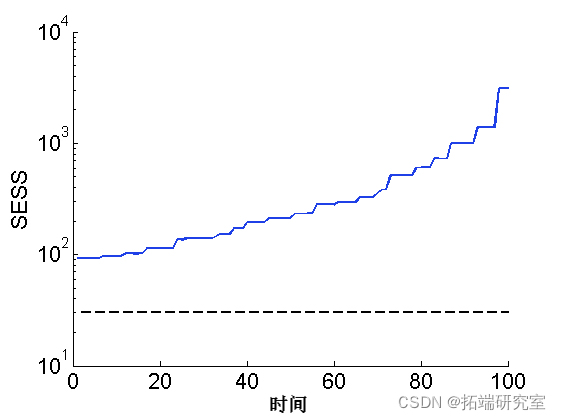
绘图平滑 ESS
sem(ess)

plot(1:tmax, 30*(tmax,1), '--k')
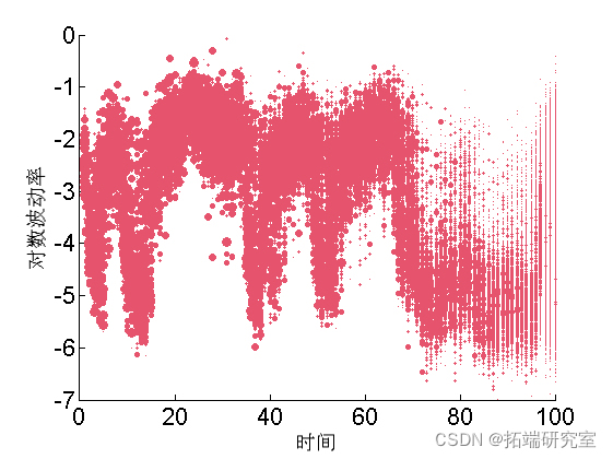
绘制加权粒子
for ttt=1:tttmax
    va = unique(outtt.x.s.vaues(ttt,:));

    wegh = arrayfun(@(x) sum(outtt.x.s.weittt(ttt, outtt.x.s.vaues(ttt,:) == x)), va);

    scatttttter(ttt*ones(size(va)), va, min(50, .5*n_parttt*wegh), 'r',...
        'markerf', 'r')
end
汇总统计
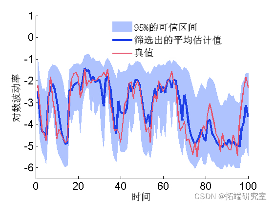
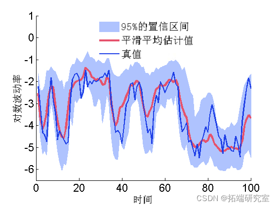
summary(out, 'pro', [.025, .975]);绘图滤波估计
mean = susmc.x.f.mean;
xfqu = susmc.x.f.quant;
h = fill([1:tmax, tmax:-1:1], [xfqu{1}; flipud(xfqu{2})], 0);

plot(1:tmax, mean,)
plot(1:tmax, data.x_true)
绘图平滑估计
mean = smcx.s.mean;
quant = smcx.s.quant;

plot(1:t_max, mean,  3)
plot(1:t_max, data.x_true, 'g')
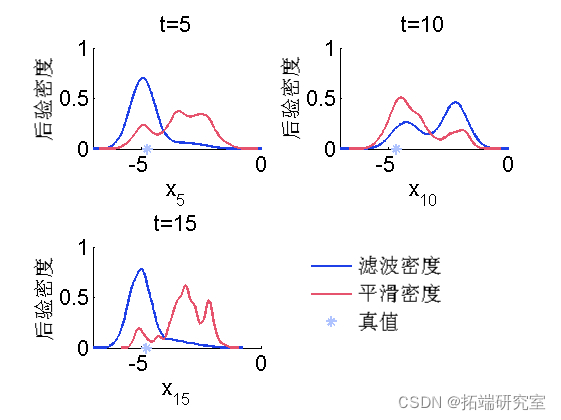
边际滤波和平滑密度
kde = density(out);
for k=1:numel(time)
    tk = time(k);
    plot(kde.x.f(tk).x, kde.x.f(tk).f);
    hold on
    plot(kde.x.s(tk).x, kde.x.s(tk).f, 'r');
    plot(data.xtrue(tk));
    box off
end
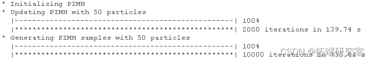
Biips 粒子独立 Metropolis-Hastings
PIMH 参数
thi= 1;
nprt = 50;
运行 PIMH
init(moel, vaibls);
upda(obj, urn, npat); % 预烧迭代
sample(obj,...
    nier, npat, 'thin', thn);
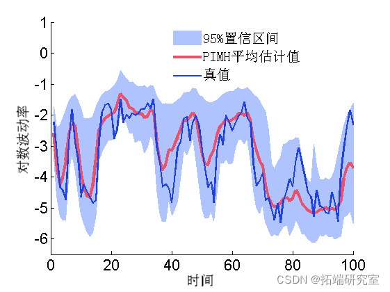
一些汇总统计
summary(out, 'prs');后均值和分位数
mean = sumx.man;
quant = su.x.qunt;

hold on
plot(1:tax, man, 'r', 'liith', 3)
plot(1:tax, xrue, 'g')
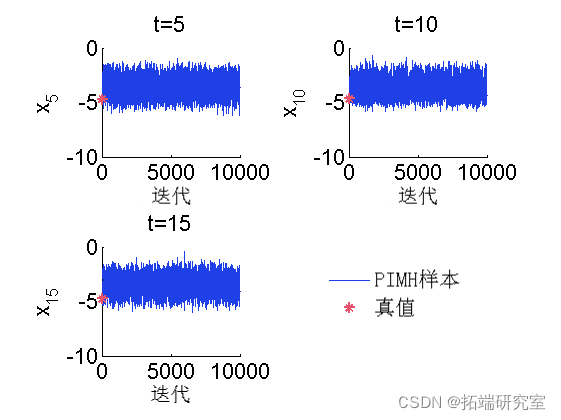
MCMC 样本的踪迹
for k=1:nmel(timndx)
    tk = tieinx(k);
    sublt(2, 2, k)
    plot(outm.x(tk, :), 'liedh', 1)
    hold on
    plot(0, d_retk), '*g');
    box off
end
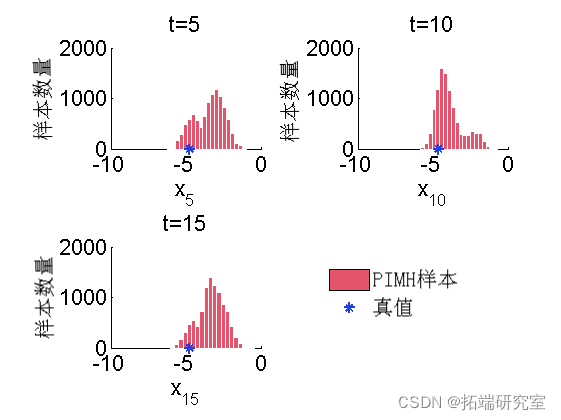
后验直方图
for k=1:numel(tim_ix)
    tk = tim_ix(k);
    subplot(2, 2, k)
    hist(o_hx(tk, :), 20);
    h = fidobj(gca, 'ype, 'ptc');    hold on
    plot(daau(k), 0, '*g');

    box off
end
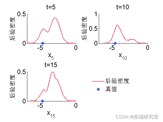
后验的核密度估计
pmh = desity(otmh);
for k=1:numel(tenx)
    tk = tim_ix(k);
    subplot(2, 2, k)
    plot(x(t).x, dpi.x(tk).f, 'r');
    hold on
    plot(xtrue(tk), 0, '*g');
    box off
end
Biips 敏感性分析
我们想研究对参数值的敏感性 
算法参数
n= 50; % 粒子数
para = {'alpha}; % 我们要研究灵敏度的参数
 % 两个分量的值网格
pvs = {A(:, B(:';
使用 SMC 运行灵敏度分析
smcs(modl, par, parvlu, npt);

绘制对数边际似然和惩罚对数边际似然率
surf(A, B, reshape(ouma_i, sizeA)
box off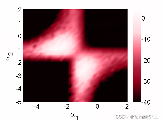


 473
473

 被折叠的 条评论
为什么被折叠?
被折叠的 条评论
为什么被折叠?
 到【灌水乐园】发言


