C++ YOLOv3推理第三讲: 模型推理

海滩游侠

已于 2024-02-19 11:52:36 修改

阅读量463

点赞数 8

分类专栏：模型部署文章标签： c++ YOLO

于 2024-01-29 23:25:00 首次发布

本文链接：https://blog.csdn.net/qq_19859865/article/details/135320423

版权

模型部署专栏收录该内容

5 篇文章 0 订阅

订阅专栏

在上一章节中，我们讨论了模型参数的加载，本文主要讨论，如何基于加载的模型实现模型的推理。

如果对于yolov3的模型结构感兴趣，那么你可能需要至少看三篇论文【4】【5】【6】

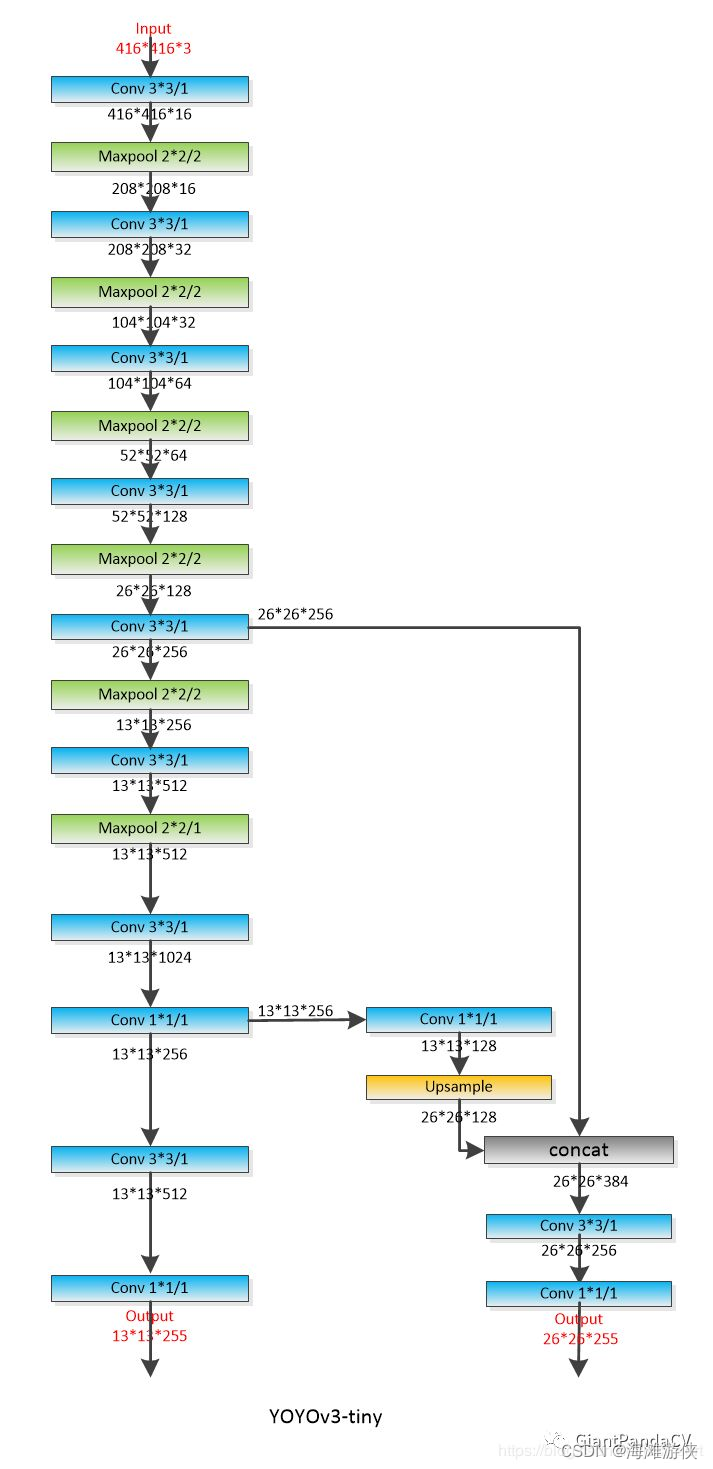
模型架构可视化

首先，梳理一下YOLOV3Tiny的模型结构，从模型结构可以看出，yolov3TIny的模型结构非常简洁。

Backbone包含卷积层，pooling层，残差链接，以及上采样层。没有其他的多余操作。

模型推理代码解读

模型推理主要调用的函数是detect(),所以，虽然这个函数很长，我们也把它展示在最后面。

    const int64_t t_start_ms = ggml_time_ms();
    detect(img, model, params.thresh, labels, alphabet);
    const int64_t t_detect_ms = ggml_time_ms() - t_start_ms;
    if (!save_image(img, params.fname_out.c_str(), 80)) {
        fprintf(stderr, "%s: failed to save image to '%s'\n", __func__, params.fname_out.c_str());
        return 1;
    }
    printf("Detected objects saved in '%s' (time: %f sec.)\n", params.fname_out.c_str(), t_detect_ms / 1000.0f);
    ggml_free(model.ctx);
    return 0;

在函数detect中，可以看到，通过ggml_init() 函数的调用，首先进行了heap上buffer的分配。然后，通过ggml_init的调用，我们进行内存的分配，并且，我们可以根据编译选项，选择是否基于cublas或者clblast或者metal进行加速。所以，目前看来，ggml_init可以实现内存的获取，以及cublas等加速器的初始化。

接下来，调用的是ggml_new_graph()。这里从名字就可以看出，涉及到图（graph）的生成，而ggml_cgraph的声明如下，网络中重要的节点会放置在其中。

在get_yolo_detections中，可以看到获得candidates 的objectness等参数的过程。

    // computation graph
    struct ggml_cgraph {
        int size;
        int n_nodes;
        int n_leafs;

        struct ggml_tensor ** nodes;
        struct ggml_tensor ** grads;
        struct ggml_tensor ** leafs;

        struct ggml_hash_set visited_hash_table;

        enum ggml_cgraph_eval_order order;

        // performance
        int     perf_runs;
        int64_t perf_cycles;
        int64_t perf_time_us;
    };

基于letterbox，我们可以对于图像进行大小的缩放，来满足模型对于输入的要求，然后成为“input”。如果仔细阅读下列代码和上图，可以发现很容易找到层之间的对应关系。

在最后，基于先验的锚点和mask信息，我们进一步处理。对应的python代码[3]可表达为：


yolo_tiny_anchors = np.array([(10, 14), (23, 27), (37, 58),
                              (81, 82), (135, 169),  (344, 319)],
                             np.float32) / 416
yolo_tiny_anchor_masks = np.array([[3, 4, 5], [0, 1, 2]])

Mask和Anchor的作用，可以参考[4]，它是基于作者提供的先验box大小。最后，经过NMS

和可视化的操作，我们完成了模型推理的全流程。

void detect(yolo_image & img, const yolo_model & model, float thresh, const std::vector<std::string> & labels, const std::vector<yolo_image> & alphabet)
{
    static size_t buf_size = 20000000 * sizeof(float) * 4;
    static void * buf = malloc(buf_size);

    struct ggml_init_params params = {
        /*.mem_size   =*/ buf_size,
        /*.mem_buffer =*/ buf,
        /*.no_alloc   =*/ false,
    };

    struct ggml_context * ctx0 = ggml_init(params);
    struct ggml_cgraph * gf = ggml_new_graph(ctx0);
    std::vector<detection> detections;

    yolo_image sized = letterbox_image(img, model.width, model.height);
    struct ggml_tensor * input = ggml_new_tensor_4d(ctx0, GGML_TYPE_F32, model.width, model.height, 3, 1);
    std::memcpy(input->data, sized.data.data(), ggml_nbytes(input));
    ggml_set_name(input, "input");

    struct ggml_tensor * result = apply_conv2d(ctx0, input, model.conv2d_layers[0]);
    print_shape(0, result);
    result = ggml_pool_2d(ctx0, result, GGML_OP_POOL_MAX, 2, 2, 2, 2, 0, 0);
    print_shape(1, result);
    result = apply_conv2d(ctx0, result, model.conv2d_layers[1]);
    print_shape(2, result);
    result = ggml_pool_2d(ctx0, result, GGML_OP_POOL_MAX, 2, 2, 2, 2, 0, 0);
    print_shape(3, result);
    result = apply_conv2d(ctx0, result, model.conv2d_layers[2]);
    print_shape(4, result);
    result = ggml_pool_2d(ctx0, result, GGML_OP_POOL_MAX, 2, 2, 2, 2, 0, 0);
    print_shape(5, result);
    result = apply_conv2d(ctx0, result, model.conv2d_layers[3]);
    print_shape(6, result);
    result = ggml_pool_2d(ctx0, result, GGML_OP_POOL_MAX, 2, 2, 2, 2, 0, 0);
    print_shape(7, result);
    result = apply_conv2d(ctx0, result, model.conv2d_layers[4]);
    struct ggml_tensor * layer_8 = result;
    print_shape(8, result);
    result = ggml_pool_2d(ctx0, result, GGML_OP_POOL_MAX, 2, 2, 2, 2, 0, 0);
    print_shape(9, result);
    result = apply_conv2d(ctx0, result, model.conv2d_layers[5]);
    print_shape(10, result);
    result = ggml_pool_2d(ctx0, result, GGML_OP_POOL_MAX, 2, 2, 1, 1, 0.5, 0.5);
    print_shape(11, result);
    result = apply_conv2d(ctx0, result, model.conv2d_layers[6]);
    print_shape(12, result);
    result = apply_conv2d(ctx0, result, model.conv2d_layers[7]);
    struct ggml_tensor * layer_13 = result;
    print_shape(13, result);
    result = apply_conv2d(ctx0, result, model.conv2d_layers[8]);
    print_shape(14, result);
    result = apply_conv2d(ctx0, result, model.conv2d_layers[9]);
    struct ggml_tensor * layer_15 = result;
    print_shape(15, result);
    result = apply_conv2d(ctx0, layer_13, model.conv2d_layers[10]);
    print_shape(18, result);
    result = ggml_upscale(ctx0, result, 2);
    print_shape(19, result);
    result = ggml_concat(ctx0, result, layer_8);
    print_shape(20, result);
    result = apply_conv2d(ctx0, result, model.conv2d_layers[11]);
    print_shape(21, result);
    result = apply_conv2d(ctx0, result, model.conv2d_layers[12]);
    struct ggml_tensor * layer_22 = result;
    print_shape(22, result);

//将layer15, layer22存入图中

    ggml_build_forward_expand(gf, layer_15);
    ggml_build_forward_expand(gf, layer_22);
    ggml_graph_compute_with_ctx(ctx0, gf, 1);

    yolo_layer yolo16{ 80, {3, 4, 5}, {10, 14, 23, 27, 37,58, 81, 82, 135, 169, 344, 319}, layer_15};
    apply_yolo(yolo16);
    get_yolo_detections(yolo16, detections, img.w, img.h, model.width, model.height, thresh);

    yolo_layer yolo23{ 80, {0, 1, 2}, {10, 14, 23, 27, 37,58, 81, 82, 135, 169, 344, 319}, layer_22};
    apply_yolo(yolo23);
    get_yolo_detections(yolo23, detections, img.w, img.h, model.width, model.height, thresh);

    do_nms_sort(detections, yolo23.classes, .45);
    draw_detections(img, detections, thresh, labels, alphabet);
    ggml_free(ctx0);
}