RNN循环神经网络 2022-1-12

人工智能基础总目录

一、 出现背景

序列问题， 输入的前后元素存在相关性，全连接神经网络无法很好的解决。wx + b

二、 RNN 模型说明

如果把上面有W的那个带箭头的圈去掉，它就变成了最普通的全连接神经网络。
x是一个向量，它表示输入层的值（这里面没有画出来表示神经元节点的圆圈）；
s是一个向量，它表示隐藏层的值（这里隐藏层面画了一个节点，你也可以想象这一层其实是多个节点，节点数与向量s的维度相同）；

U是输入层到隐藏层的权重矩阵，o也是一个向量，它表示输出层的值；
V是隐藏层到输出层的权重矩阵。

循环神经网络的隐藏层的值s不仅仅取决于当前这次的输入x，还取决于上一次隐藏层的值s。权重矩阵 W就是隐藏层上一次的值作为这一次的输入的权重。

RNN 特别容易发生梯度消失或梯度爆炸的问题， Loss 对wi 求偏导， 求导边长了，改善方式 LSTM 模型。

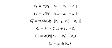
三、 LSTM 模型

解决梯度消失方案

• 存在一些单元，输出对输入是一个常数 保证有一些数据不会变的特别小，
• 能否设置阀门控制， ht-1 到 ht 不重要时，偏导比较小接近于0，重要时大于一个常数。这个阀门可以通过学习得到。Gate Informaion Control
  

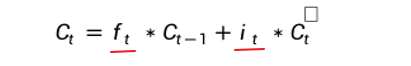
3.1 PEEPHOLE的LSTM

改进版本，将Ct-1 也增加到对Ft 的影响中：

四、 GRU

2014年提出 Gated Recurrent Unit ， LSTM 的简化版本。

在LSTM 中： 当过去的影响比较大时，ft 大 it 小， 所以将 ft = 1 - it
将 LSTM 的三个参数 f i o 简化为 Zt 和 rt， 对过拟合，数据量不够的问题有很大帮助。

五、存在问题

LSTM 最大问题， 假设x 是100个，必须一个个来训练，输入层上无法发挥并行计算的能力。
数据量不大时还是有效的。

六、 LSTM 代码实践

使用 LSTM 拟合正余弦函数

6.1 构造数据集

这一模块将使用 numpy 构造时间序列数据，主要有两个步骤：

定义正弦函数 (余弦函数)
选定历史数据窗口大小构造时序数据

# 导入必要的库
import numpy as np  # 构建数据
# 搭建模型
from tensorflow.keras.models import Sequential
from tensorflow.keras.layers import Input
from tensorflow.keras.layers import LSTM
from tensorflow.keras.layers import Dense

from tqdm import tqdm  # 打印进度条

import matplotlib.pyplot as plt  # 可视化
%matplotlib inline

def ground_func(x):
    y = np.sin(x)
    return y

def build_data(sequence_data, n_steps):
    # init 
    X, y = [], []
    
    seq_len = len(sequence_data)
    for start_idx in tqdm(range(seq_len), total=seq_len):
        end_idx = start_idx + n_steps
        
        if end_idx >= seq_len:
            break
        # hits:
        #     1. sequence data in slice(start_idx, end_idx) as current x
        #     2. end index data as current y
        cur_x = sequence_data[start_idx: end_idx]
        cur_y = sequence_data[end_idx]
        X.append(cur_x)
        y.append(cur_y)
        
    X = np.array(X)
    y = np.array(y)
    
    # *X.shape get number of examples and n_steps, but LSTM need inputs like (batch, n_steps, n_features),
    # here we only have 1 feature
    X = X.reshape(*X.shape, 1)
        
    return X, y


# 构造原始正弦/余弦函数序列
xaxis = np.arange(-50 * np.pi, 50 * np.pi, 0.1)
sequence_data = ground_func(xaxis)
len(sequence_data)  # 查看数据量


# 取 1000 个数据进行可视化
plt.figure(figsize=(20, 8))
plt.plot(xaxis[:1000], sequence_data[:1000]);

n_steps = 20  # 可以尝试更改
X, y = build_data(sequence_data, n_steps)
X.shape, y.shape  # 查看 X, y 的维度信息

6.2 搭建模型

本模块基于 keras 中的 LSTM、Dense 层搭建时序模型，需要注意以下几点：

• 选择合适的 hidden size
• 选择合适的激活函数，比如 relu、tanh
• 优化器选择 sgd、adam 等等
• 损失函数选择交叉熵损失函数(cross_entropy) 还是均方误差(mse) 等等

def create_model():
    """Build a LSTM model fit sine/cosine function.
    
    hints: 
        1. a LSTM fit time pattern (ref: https://www.tensorflow.org/api_docs/python/tf/keras/layers/LSTM)
        2. a Dense for regression (ref: https://www.tensorflow.org/api_docs/python/tf/keras/layers/Dense)
    """
    ######## your code ~ 5 line ########
    model = Sequential()
    model.add(Input(shape=(20, 1)))
    model.add(LSTM(32, activation='tanh'))
    model.add(Dense(1, activation='tanh'))
    model.compile(optimizer='adam', loss='mse')
    ######## your code ########
    return model

# 初始化模型并打印相关信息
model = create_model()
model.summary()

6.3. 模型训练 与预测

history = model.fit(X, y, batch_size=32, epochs=25, verbose=1)
plt.plot(history.history['loss'], label="loss")
plt.legend(loc="upper right")  # 画出损失图像

def test_function(x):
    y = np.sin(x)
    return y

test_xaxis = np.arange(0, 10 * np.pi, 0.1)

test_sequence_data = test_function(test_xaxis)

# 利用初始的 n_steps 个历史数据开始预测，后面的数据依次利用预测出的数据作为历史数据进行进一步预测
y_preds = test_sequence_data[:n_steps]

# 逐步预测
for i in tqdm(range(len(test_xaxis) - n_steps)):
    model_input = y_preds[i: i + n_steps]
    model_input = model_input.reshape((1, n_steps, 1))
    ######## your code ~ 1 line ########
    y_pred = model.predict(model_input, verbose=0)
    ######## your code ########
    y_preds = np.append(y_preds, y_pred)

# 可视化
plt.figure(figsize=(10, 8))
plt.plot(test_xaxis[n_steps:], y_preds[n_steps:], label="predicitons")
plt.plot(test_xaxis, test_sequence_data, label="ground truth")
plt.plot(test_xaxis[:n_steps], y_preds[:n_steps], label="initial sequence", color="red")
plt.legend(loc='upper left')
plt.ylim(-2, 2)
plt.show()