同花顺Supermind量化交易 金融时间序列2--GARCH模型 附源代码

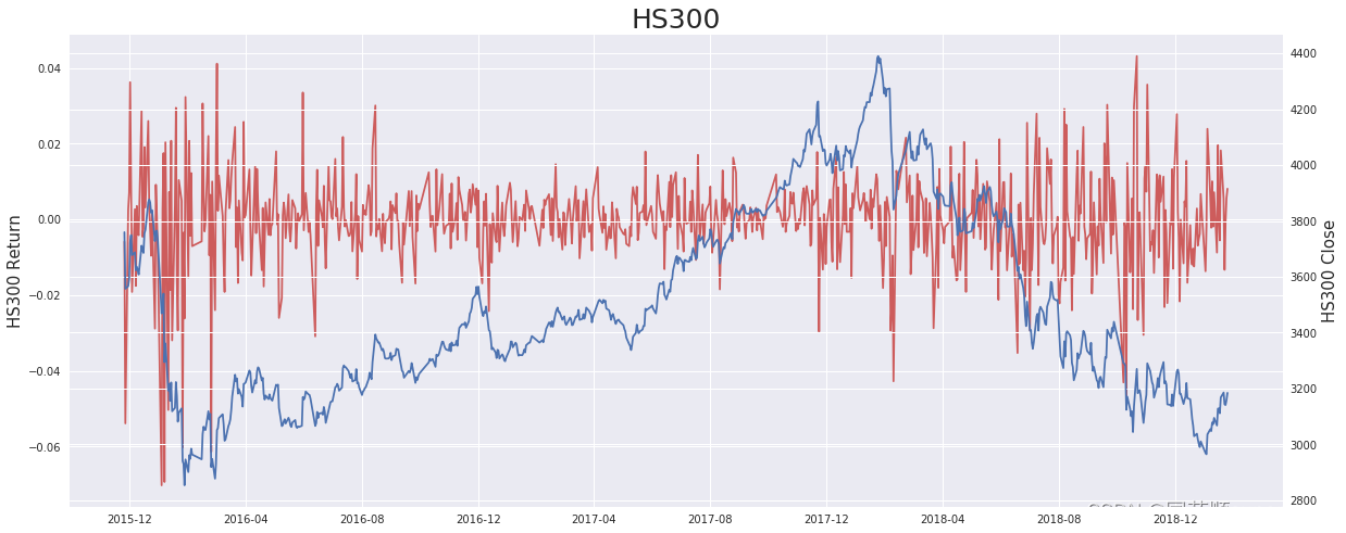
从金融时间序列的角度，以 沪深 300的收益作为研究标的，使用GARCH等衍生模型进行探讨和对比，并尝试对价格和波动率进行一定的拟合和预测。

金融时间序列（二）

作者：邱吉尔

1. 输入库包

In [1]:

from scipy import stats
import statsmodels.api as sm
import numpy as np
import pandas as pd
import matplotlib.pyplot as plt
import seaborn as sns
plt.style.use('seaborn')
import arch

2. 取出数据

In [2]:

HS300_close=get_price(['000300.SH'], '20151125', '20190125', '1d', ['close'], True, None,is_panel=1)['close']
HS300_close.columns=['HS300_close']
HS300_close['return']=HS300_close['HS300_close'].pct_change()
HS300_close.dropna(inplace=True)
datetime=pd.to_datetime(HS300_close.index)
fig,ax=plt.subplots(figsize=(20,8))
rect1=ax.plot(datetime,HS300_close['return'],color='IndianRed')
ax.set_ylabel('HS300 Return',size=15)
ax=ax.twinx()
rect2=ax.plot(datetime,HS300_close['HS300_close'])
ax.set_ylabel('HS300 Close',size=15)
plt.title('HS300',size=25)

Out[2]:

<matplotlib.text.Text at 0x7fca33a75f60>

3. GARCH 模型

对于一个对数收益率序列rt，令：

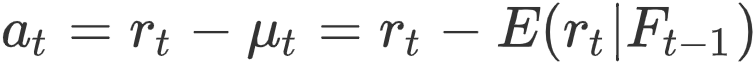
如果at满足以下式子：
 

 

 

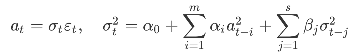
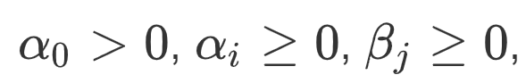
则称at服从GARCH模型,其中,{ϵt} 是均值为0,方差为1的独立同分布随机变量序列.

1. 数据集分类，GARCH模型拟合

In [142]:

train_GARCH =HS300_close['return'][:-30]
test_GARCH = HS300_close['return'][-30:]
am_GARCH = arch.arch_model(train_GARCH, mean='AR', lags=14, vol='GARCH') 
res_GARCH = am_GARCH.fit()

Iteration:      1,   Func. Count:     20,   Neg. LLF: -2322.719676744772
Iteration:      2,   Func. Count:     48,   Neg. LLF: -2324.118636827964
Iteration:      3,   Func. Count:     78,   Neg. LLF: -2323.6843401398555
Iteration:      4,   Func. Count:    108,   Neg. LLF: -2324.1246848237706
Iteration:      5,   Func. Count:    133,   Neg. LLF: -2324.1264594013755
Iteration:      6,   Func. Count:    163,   Neg. LLF: -2316.849320551835
Iteration:      7,   Func. Count:    193,   Neg. LLF: -2328.0083395660868
Iteration:      8,   Func. Count:    223,   Neg. LLF: -2327.4637810024988
Iteration:      9,   Func. Count:    251,   Neg. LLF: -2328.0231532432426
Iteration:     10,   Func. Count:    281,   Neg. LLF: -2325.763855473391
Iteration:     11,   Func. Count:    311,   Neg. LLF: -2328.0188277867
Iteration:     12,   Func. Count:    338,   Neg. LLF: -2328.024075604725
Positive directional derivative for linesearch    (Exit mode 8)
            Current function value: -2328.024084172148
            Iterations: 16
            Function evaluations: 338
            Gradient evaluations: 12

/opt/conda/lib/python3.5/site-packages/arch/univariate/base.py:517: ConvergenceWarning: 
The optimizer returned code 8. The message is:
Positive directional derivative for linesearch
See scipy.optimize.fmin_slsqp for code meaning.

  ConvergenceWarning)

In [15]:

res_GARCH.summary()

Out[15]:

AR - GARCH Model Results

Dep. Variable:	return	R-squared:	0.071
Mean Model:	AR	Adj. R-squared:	0.053
Vol Model:	GARCH	Log-Likelihood:	2328.02
Distribution:	Normal	AIC:	-4620.05
Method:	Maximum Likelihood	BIC:	-4537.35
		No. Observations:	731
Date:	Tue, Feb 12 2019	Df Residuals:	713
Time:	10:13:35	Df Model:	18

Mean Model

	coef	std err	t	P>|t|	95.0% Conf. Int.
Const	4.3118e-04	3.001e-04	1.437	0.151	[-1.570e-04,1.019e-03]
return[1]	-0.0426	3.569e-02	-1.193	0.233	[ -0.113,2.737e-02]
return[2]	0.0299	3.594e-02	0.832	0.406	[-4.054e-02, 0.100]
return[3]	0.0652	4.003e-02	1.628	0.103	[-1.327e-02, 0.144]
return[4]	-0.0582	3.710e-02	-1.568	0.117	[ -0.131,1.454e-02]
return[5]	-0.0575	3.989e-02	-1.441	0.150	[ -0.136,2.072e-02]
return[6]	-0.0528	3.239e-02	-1.631	0.103	[ -0.116,1.066e-02]
return[7]	0.0393	3.921e-02	1.002	0.316	[-3.756e-02, 0.116]
return[8]	-0.0306	3.370e-02	-0.908	0.364	[-9.665e-02,3.545e-02]
return[9]	0.0874	3.520e-02	2.484	1.298e-02	[1.845e-02, 0.156]
return[10]	-7.3447e-03	3.654e-02	-0.201	0.841	[-7.897e-02,6.428e-02]
return[11]	0.0228	3.433e-02	0.664	0.507	[-4.448e-02,9.008e-02]
return[12]	-0.0516	3.641e-02	-1.418	0.156	[ -0.123,1.972e-02]
return[13]	0.0646	3.598e-02	1.796	7.250e-02	[-5.901e-03, 0.135]
return[14]	-0.1405	3.224e-02	-4.356	1.323e-05	[ -0.204,-7.727e-02]

Volatility Model

	coef	std err	t	P>|t|	95.0% Conf. Int.
omega	2.6238e-06	4.121e-12	6.367e+05	0.000	[2.624e-06,2.624e-06]
alpha[1]	0.0500	1.510e-02	3.312	9.261e-04	[2.042e-02,7.960e-02]
beta[1]	0.9300	1.063e-02	87.477	0.000	[ 0.909, 0.951]

In [16]:

res_GARCH.params

Out[16]:

Const         0.000431
return[1]    -0.042592
return[2]     0.029893
return[3]     0.065190
return[4]    -0.058172
return[5]    -0.057475
return[6]    -0.052824
return[7]     0.039286
return[8]    -0.030600
return[9]     0.087443
return[10]   -0.007345
return[11]    0.022798
return[12]   -0.051641
return[13]    0.064623
return[14]   -0.140464
omega         0.000003
alpha[1]      0.050010
beta[1]       0.930000
Name: params, dtype: float64

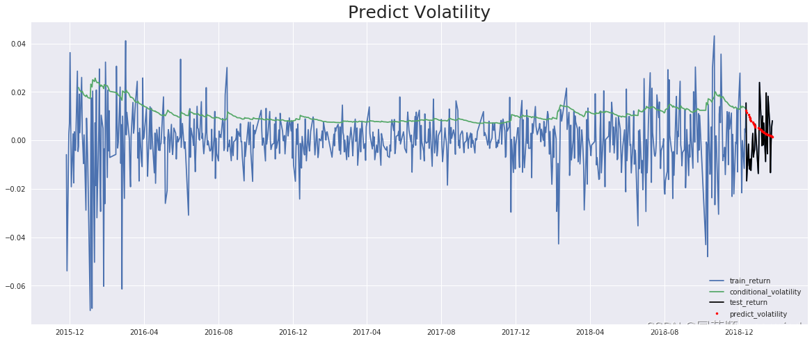
2. GARCH模型预测
前面ARCH模型，我们用来预测了收益率，然而直接预测收益率准确度并不是很高，因此很多时候我们主要用来预测波动率.

In [22]:

resid=res_GARCH.resid[-14:]                 #取出过去14天的残差at
params=np.array(res_GARCH.params[1:15])               #取出均值方程所有系数    
w_params=params[::-1]                       #倒转系数方向
w_params.dot(resid[-14:])

for i in range(30):
    resid_new=test_GARCH.iloc[i]-(res_GARCH.params[0]+w_params.dot(resid[-14:]))
    resid=np.append(resid,resid_new)
resid_final=resid[-30:]
resid_final_square=resid_final**2
resid_final_square

Out[22]:

array([1.31265182e-04, 4.24223468e-04, 2.34277150e-05, 8.61572516e-05,
       7.61609044e-05, 9.93121008e-05, 6.07929980e-05, 9.97465719e-08,
       3.17377608e-05, 1.50034013e-04, 7.63315088e-06, 1.93504633e-05,
       1.31637564e-04, 1.60983709e-05, 6.62189736e-04, 2.51275329e-05,
       1.20477057e-05, 3.81599502e-05, 3.29924979e-06, 6.78092403e-05,
       8.81824346e-05, 3.51298854e-04, 1.00565226e-06, 6.70353037e-05,
       2.03613211e-04, 6.43136485e-05, 1.87956839e-04, 1.15415026e-05,
       4.33123654e-05, 1.57135491e-04])

In [54]:

volatility=res_GARCH.conditional_volatility[-1:]
for i in range(30):
    new_volatility=0.000003+0.05001*resid_final_square[i]+0.93*volatility[-1]
    volatility=np.append(volatility,new_volatility)
    
pre_volatility=volatility[-30:]
pre_volatility

Out[54]:

array([0.01227059, 0.01143586, 0.01063952, 0.00990207, 0.00921573,
       0.0085786 , 0.00798413, 0.00742825, 0.00691286, 0.00643946,
       0.00599208, 0.0055766 , 0.00519582, 0.00483592, 0.00453352,
       0.00422043, 0.00392861, 0.00365851, 0.00340558, 0.00317358,
       0.00295884, 0.00277229, 0.00258128, 0.00240694, 0.00225164,
       0.00210024, 0.00196562, 0.00183161, 0.00170856, 0.00159982])

In [55]:

test_GARCH

Out[55]:

2018-12-13    0.015481
2018-12-14   -0.016704
2018-12-17   -0.001489
2018-12-18   -0.010366
2018-12-19   -0.011923
2018-12-20   -0.007670
2018-12-21   -0.012395
2018-12-24    0.002906
2018-12-25   -0.006885
2018-12-26   -0.005054
2018-12-27   -0.003840
2018-12-28    0.006737
2019-01-02   -0.013658
2019-01-03   -0.001580
2019-01-04    0.023958
2019-01-07    0.006070
2019-01-08   -0.002161
2019-01-09    0.010097
2019-01-10   -0.001881
2019-01-11    0.007190
2019-01-14   -0.008722
2019-01-15    0.019625
2019-01-16    0.000211
2019-01-17   -0.005509
2019-01-18    0.018242
2019-01-21    0.005512
2019-01-22   -0.013284
2019-01-23   -0.000720
2019-01-24    0.005644
2019-01-25    0.008132
Name: return, dtype: float64

In [93]:

HS300_close.index=pd.to_datetime(HS300_close.index)
res_GARCH.conditional_volatility.index=pd.to_datetime(res_GARCH.conditional_volatility.index)

plt.figure(figsize=(20,8))
plt.plot(HS300_close['return'],label='train_return')
plt.plot(res_GARCH.conditional_volatility,label='conditional_volatility')
x=test_GARCH.index
plt.plot(test_GARCH,'black',label='test_return')
plt.plot(x,pre_volatility,'.r',label='predict_volatility')
plt.title('Predict Volatility',size=25)
plt.legend()

Out[93]:

<matplotlib.legend.Legend at 0x7fc9cd798358>

In [ ]:

查看以上策略详细请 到 supermind量化交易官网查看：金融时间序列2--GARCH模型附源代码