


1.单变量线性回归
> y<-c(5,7,9,11,16,20)
> x<-c(1,2,3,4,7,9)
> lsfit(x,y)
$coefficients
Intercept         X
 3.338028  1.845070

$residuals
[1] -0.18309859 -0.02816901  0.12676056  0.28169014 -0.25352113  0.05633803
...
用lm函数可以进行更加详细的回归分析。
> lm(y~x)->xy
> summary(xy)#分析一下拟合效果
Call:
lm(formula = y ~ x)
Residuals:
1 2 3 4 5 6
-0.18310 -0.02817 0.12676 0.28169 -0.25352 0.05634
Coefficients:
Estimate Std. Error t value Pr(>|t|)
(Intercept) 3.33803 0.16665 20.03 3.67e-05 ***
x 1.84507 0.03227 57.17 5.60e-07 ***
---
Signif. codes: 0 ‘***’ 0.001 ‘**’ 0.01 ‘*’ 0.05 ‘.’ 0.1 ‘ ’ 1
Residual standard error: 0.222 on 4 degrees of freedom
Multiple R-squared: 0.9988, Adjusted R-squared: 0.9985
F-statistic: 3269 on 1 and 4 DF, p-value: 5.604e-07
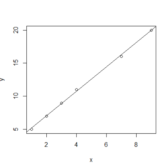
> plot(x,y)
> abline(lm(y~x))
结果如下:
在Coeffients栏中各个参数的意义如下:
Estimate:斜率与截距的估计值。
Std.Error:斜率与截距的估计标准差。
t value:斜率与截距的假设检验的t值。
Pr(>|t|):与显著性水平比较,决定是否接受该假设检验。
在Coeffients每行最后一列的*号体现线性关系是否强,取值为0~3,线性关系越强,*号数量越多。
2.多元线性回归
多元线性回归仍然可以使用lm函数分析,只不过增加了若干自变量。
如在1的基础上增加x2:
> x2<-c(6,8,10,12,16,20)
> lm(y~x+x2)->xy2
> summary(xy2)

Call:
lm(formula = y ~ x + x2)

Residuals:
         1          2          3          4          5          6
-7.495e-16  9.195e-16  4.172e-17 -2.117e-16  1.839e-16 -1.839e-16

Coefficients:
             Estimate Std. Error   t value Pr(>|t|)
(Intercept) 1.000e+00  3.787e-15 2.640e+14   <2e-16 ***
x           1.000e+00  1.359e-15 7.357e+14   <2e-16 ***
x2          5.000e-01  8.019e-16 6.236e+14   <2e-16 ***
---
Signif. codes:  0 ‘***’ 0.001 ‘**’ 0.01 ‘*’ 0.05 ‘.’ 0.1 ‘ ’ 1

Residual standard error: 7.121e-16 on 3 degrees of freedom
Multiple R-squared:      1,     Adjusted R-squared:      1
F-statistic: 1.591e+32 on 2 and 3 DF,  p-value: < 2.2e-16
3.非线性回归
使用nls函数,应用最小二乘法,实现非线性回归。
> x<-c(1,2,3,4,7,8,9)
> y<-100 + 10*exp(x/2) + rnorm(x)#假设回归方程已知
> nlmod<- nls(y~ Const + A * exp(B*x))
> summary(nlmod)

Formula: y ~ Const + A * exp(B * x)

Parameters:
       Estimate Std. Error t value Pr(>|t|)
Const 99.215566   0.738878  134.28 1.84e-08 ***
A     10.194798   0.156569   65.11 3.33e-07 ***
B      0.498002   0.001691  294.50 7.98e-10 ***
---
Signif. codes:  0 ‘***’ 0.001 ‘**’ 0.01 ‘*’ 0.05 ‘.’ 0.1 ‘ ’ 1

Residual standard error: 0.9671 on 4 degrees of freedom

Number of iterations to convergence: 8
Achieved convergence tolerance: 2.197e-08

#绘制拟合效果图
> plot(x,y,main = "nls(o)")
> curve(100 + 10*exp(x/2),col = 4,add = TRUE)
> lines(x,predict(nlmod),col =2,type = 'b')
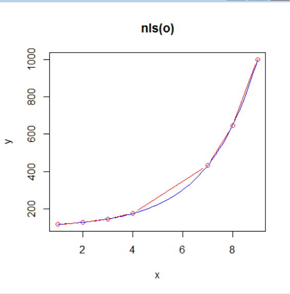
虽然样本数据量很少,但是拟合的效果还不错。
增加数据点:
> x<-seq(1,10,0.1)
> y<-100 + 10*exp(x/2) + rnorm(x)
> nlmod<- nls(y~ Const + A * exp(B*x))
> plot(x,y,main = "nls(o)")
> curve(100 + 10*exp(x/2),col = 4,add = TRUE)
> lines(x,predict(nlmod),col =2,type = 'b')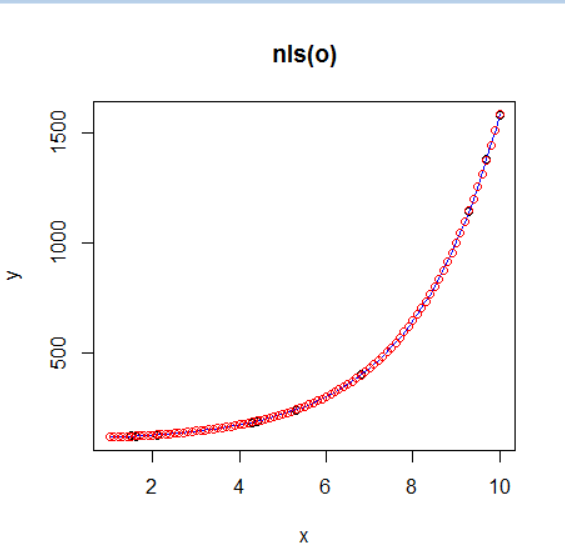
与实际回归方程非常接近了。
接下来扩大随机数的范围,增大残差,使其更加接近真实环境。
> x<-seq(1,10,0.1)
> y<-100 + 10*exp(x/2) + rnorm(x)*100
> nlmod<- nls(y~ Const + A * exp(B*x))
> plot(x,y,main = "nls(o)")
> curve(100 + 10*exp(x/2),col = 4,add = TRUE)
> lines(x,predict(nlmod),col =2,type = 'b')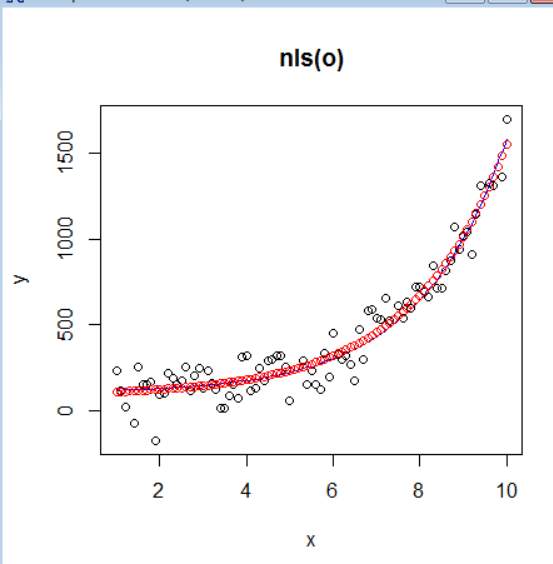


 2万+
2万+

 被折叠的 条评论
为什么被折叠?
被折叠的 条评论
为什么被折叠?
 到【灌水乐园】发言


