用R语言进行数据分析

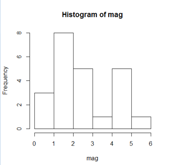
用美国地震台网公布的全球2013年5月20日22点到24点发生的所有地震的震级数据实验。

> mag<-c(1.6,0.9,2.1,2.2,2.3,1.7,1.3,1.6,4.7,1.2,0.9,4.7,0.6,5.3,1.1,4.8,4,4.2,4.6,1.3,2.1,1.5,3)
> mag
 [1] 1.6 0.9 2.1 2.2 2.3 1.7 1.3 1.6 4.7 1.2 0.9 4.7 0.6 5.3 1.1 4.8 4.0 4.2 4.6 1.3 2.1 1.5 3.0
 > factor(cut(mag,5))#建立因子
 [1] (1.54,2.48]  (0.595,1.54] (1.54,2.48]  (1.54,2.48]  (1.54,2.48]  (1.54,2.48]  (0.595,1.54]
 [8] (1.54,2.48]  (4.36,5.3]   (0.595,1.54] (0.595,1.54] (4.36,5.3]   (0.595,1.54] (4.36,5.3]  
[15] (0.595,1.54] (4.36,5.3]   (3.42,4.36]  (3.42,4.36]  (4.36,5.3]   (0.595,1.54] (1.54,2.48] 
[22] (0.595,1.54] (2.48,3.42] 
Levels: (0.595,1.54] (1.54,2.48] (2.48,3.42] (3.42,4.36] (4.36,5.3]
> factor(cut(mag,5))->magfactor#统计因子频率
> table(magfactor)
magfactor
(0.595,1.54]  (1.54,2.48]  (2.48,3.42]  (3.42,4.36]   (4.36,5.3] 
           8            7            1            2            5 

#绘制直方图
> hist(mag,breaks = 5)

下面读取地震文件进行分析:

> read.table("F:/Machine Learning/R Basic/eqweek.csv",header = TRUE,sep = ",")->earthquake
                          DateTime Latitude Longitude Depth Magnitude MagType NbStations
1    2013-05-20T23:57:12.000+00:00   63.450  -148.291   5.5       1.6      Ml         NA
2    2013-05-20T23:52:59.000+00:00   61.337  -152.069  81.4       2.1      Ml         NA
3    2013-05-20T23:49:15.100+00:00   19.990  -155.426  38.2       2.2      Md         NA
4    2013-05-20T23:46:36.000+00:00   60.498  -142.974   4.2       2.3      Ml         NA
5    2013-05-20T23:44:07.000+00:00   64.997  -147.444    NA       1.7      Ml         NA
...

#画出直方图分析
> hist(earthquake$Magnitude,5)     

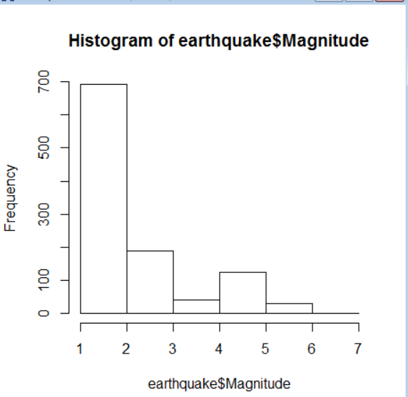
要精确分析频率大小需要进行因子频率分析:

> table(factor(cut(earthquake$Magnitude,5)))

(0.995,2.1]   (2.1,3.2]   (3.2,4.3]   (4.3,5.4]  (5.4,6.51] 
        720         178          41         126          10 

下面分析一下地震深度:

> attach(earthquake)
> summary(Depth)
   Min. 1st Qu.  Median    Mean 3rd Qu.    Max.    NA's 
   0.10    5.80   12.15   30.82   38.00  630.70      39 

作出Magnitude和Depth的散点图分析一下:

> plot(Depth,Magnitude,main = "Magnitude和Depth的关系")

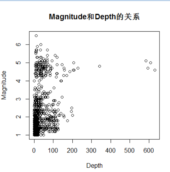
好像并没有什么关系，只能说当Depth大于了300后Magnitude在5左右，而当Depth小于300时，Magnitude取值不确定。

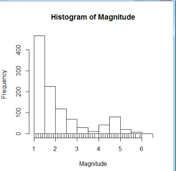
下面绘制一下有数据点的震级直方图：

> hist(Magnitude)
> rug(Magnitude)

用五分位数法分析下Magnitude和Depth

> fivenum(Magnitude)
[1] 1.0 1.3 1.7 2.5 6.5
> fivenum(Depth)
[1]   0.10   5.80  12.15  38.00 630.70

学过统计学就知道，累积分布函数描述了随机变量X的概率分布，R语言通过ecdf函数计算累积分布:

> ecdf(Magnitude)->mag_ecdf
> mag_ecdf
Empirical CDF 
Call: ecdf(Magnitude)
 x[1:50] =      1,    1.1,    1.2,  ...,      6,    6.5
> plot(mag_ecdf,do.points = FALSE,verticals = TRUE)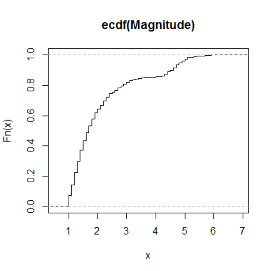

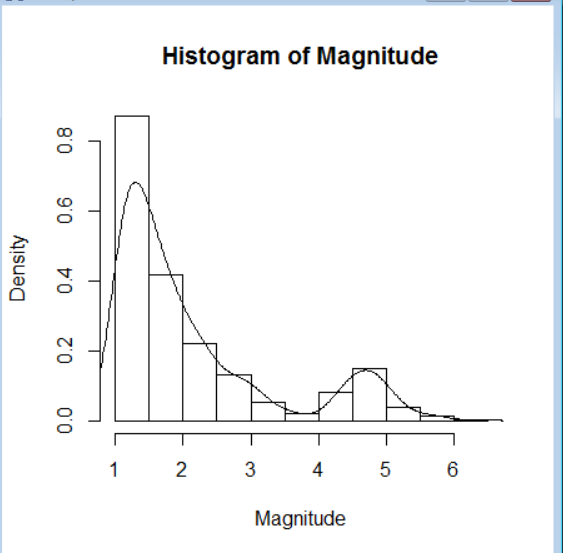
绘制一下核密度直方图(hist()函数指定参数prob = TRUE)和核密度曲线(用density进行核密度估计)

> hist(Magnitude,prob = TRUE)
> lines(density(Magnitude))