学习笔记|Pytorch使用教程14(损失函数(一))

最新推荐文章于 2024-04-09 17:09:52 发布

NotFound1911

最新推荐文章于 2024-04-09 17:09:52 发布

阅读量402

点赞数

分类专栏： Pytorch 自学文章标签： pytorch 损失函数

本文链接：https://blog.csdn.net/qq_24739717/article/details/102901199

版权

自学同时被 2 个专栏收录

78 篇文章 17 订阅

订阅专栏

Pytorch

39 篇文章 24 订阅

订阅专栏

学习笔记|Pytorch使用教程14

本学习笔记主要摘自“深度之眼”，做一个总结，方便查阅。
使用Pytorch版本为1.2

损失函数概念
交叉熵损失函数
NLL/BCE/BCEWithLogits Loss
作业

一.损失函数概念

在这里插入图片描述
损失函数:衡量模型输出与真实标签的差异

损失函数(Loss Function) :
$Loss=f\left(y^{\wedge}, y\right)$
代价函数(Cost Function) :
$\cos t=\frac{1}{N} \sum_{i}^{N} f\left(y_{i}^{\wedge}, y_{i}\right)$
目标函数(Objective Function) :
$O b j = C o s t + R e g u l a r i z a t i o n$

size_average和reduce被舍弃。

测试代码：
完整代码见
学习笔记|Pytorch使用教程09(模型创建与nn.Module)

......
# 参数设置
......
# ============================ step 1/5 数据 ============================
......

# 构建MyDataset实例
......
# 构建DataLoder
......
# ============================ step 2/5 模型 ============================
......
# ============================ step 3/5 损失函数 ============================
loss_functoin = nn.CrossEntropyLoss()                                                   # 选择损失函数
# ============================ step 4/5 优化器 ============================
 # 选择优化器
 # 设置学习率下降策略
 .......
# ============================ step 5/5 训练 ============================
......
for epoch in range(MAX_EPOCH):
......
    for i, data in enumerate(train_loader):
        # forward
		......
        # backward
        optimizer.zero_grad()
        loss = loss_functoin(outputs, labels)
        loss.backward()
        # update weights
		......
        # 统计分类情况
        # 打印训练信息
		......

在loss_functoin = nn.CrossEntropyLoss()和loss = loss_functoin(outputs, labels)处设置断点，进行debug了解其机制。
首先debug到loss_functoin = nn.CrossEntropyLoss()，并进入(step into)。


class CrossEntropyLoss(_WeightedLoss):
    r"""This criterion combines :func:`nn.LogSoftmax` and 
	.......
    Examples::

        >>> loss = nn.CrossEntropyLoss()
        >>> input = torch.randn(3, 5, requires_grad=True)
        >>> target = torch.empty(3, dtype=torch.long).random_(5)
        >>> output = loss(input, target)
        >>> output.backward()
    """
    __constants__ = ['weight', 'ignore_index', 'reduction']

    def __init__(self, weight=None, size_average=None, ignore_index=-100,
                 reduce=None, reduction='mean'):
        super(CrossEntropyLoss, self).__init__(weight, size_average, reduce, reduction)
        self.ignore_index = ignore_index

    def forward(self, input, target):
        return F.cross_entropy(input, target, weight=self.weight,
                               ignore_index=self.ignore_index, reduction=self.reduction)

进入(step into):super(CrossEntropyLoss, self).__init__(weight, size_average, reduce, reduction)

class _WeightedLoss(_Loss):
    def __init__(self, weight=None, size_average=None, reduce=None, reduction='mean'):
        super(_WeightedLoss, self).__init__(size_average, reduce, reduction)
        self.register_buffer('weight', weight)

_WeightedLoss继承于 _Loss
进行进入(step into):super(_WeightedLoss, self).__init__(size_average, reduce, reduction)

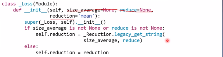
class _Loss(Module):
    def __init__(self, size_average=None, reduce=None, reduction='mean'):
        super(_Loss, self).__init__()
        if size_average is not None or reduce is not None:
            self.reduction = _Reduction.legacy_get_string(size_average, reduce)
        else:
            self.reduction = reduction

_Loss 又继承于 Module。
接下来继续debug，进入:loss_functoin = nn.CrossEntropyLoss()
在这里插入图片描述
进入:result = self.forward(*input, **kwargs)

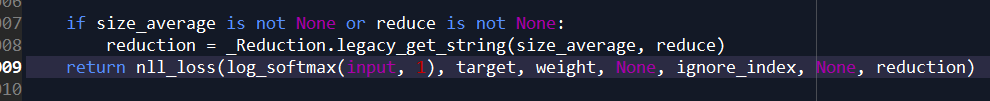
这里调用了F.cross_entropy，在该处进入(step into)
进入cross_entropy中，对reduction进行判断并进行计算。

二.交叉熵损失函数

在这里插入图片描述
交叉熵=信息熵+相对熵
$H(P, Q)=D_{K L}(P, Q)+H(P)$

交叉熵:衡量两个分布的相似度。
$\mathrm{H}(\boldsymbol{P}, \boldsymbol{Q})=-\sum_{i=1}^{N} P\left(x_{i}\right) \log Q\left(x_{i}\right)$
自信息:衡量单个输出单个事件的不确定性。
$1(x)=-\log [p(x)]$
熵:又称之为信息熵，用来描述事件的不确定性，会对自信息求期望。
$\mathrm{H}(\mathrm{P})=E_{x \sim p}[I(x)]=-\sum_{i}^{N} P\left(x_{i}\right) \log P\left(x_{i}\right)$
相对熵: 又称之为KL散度，用来衡量两个分布之间的距离、差异。
$\begin{aligned} D_{K L}(P, Q) &=E_{x \sim p}\left[\log \frac{p(x)}{Q(x)}\right] \\ &=E_{x \cdot p}[\log P(x)-\log Q(x)] \\ &=\sum_{l=1}^{N} P\left(x_{l}\right)\left[\log P\left(x_{l}\right)-\log Q\left(x_{l}\right)\right] \\ &=\sum_{l=1}^{N} P\left(x_{l}\right) \log P\left(x_{i}\right)-\sum_{i=1}^{N} P\left(x_{i}\right) \log Q\left(x_{i}\right) \\ &=H(P, Q)-H(P) \end{aligned}$

$P$ 是一个真实的概率分布(训练集、样本分布)， $Q$ 是模型的分布。优化交叉熵，相当于优化相对熵。由于训练集是固定的， $H (P)$ 是固定的，是一个常数。在做优化的时候，常数是可以忽略掉的。
1.nn.CrossEntropyLoss
功能: nn. LogSoftmax()（数据进行归一化）与nn. NLLLoss()结合，进行交叉熵计算
在这里插入图片描述
主要参数:

weight:各类别的loss设置权值
ignore_index: 忽略某个类别
reduction :计算模式，可为none/sum/mean
none-逐个元素计算
sum-所有元素求和，返回标量
mean-加权平均，返回标量

相关公式：
$\mathrm{H}(\boldsymbol{P}, \boldsymbol{Q})=-\sum_{i=1}^{N} \boldsymbol{P}\left(\boldsymbol{x}_{i}\right) \log \boldsymbol{Q}\left(\boldsymbol{x}_{i}\right)$
$\operatorname{loss}(x, \text { class })=-\log \left(\frac{\exp (x[\text { class }])}{\sum_{j} \exp (x[j])}\right)=-x[\text { class }]+\log \left(\sum_{j} \exp (x(j])\right)$
$\operatorname{loss}(x, \text { class })=$ weight $[\text {class}]\left(-x[\text {class}]+\log \left(\sum_{j} \exp (x[\boldsymbol{y}])\right)\right)$

测试代码：

import torch
import torch.nn as nn
import torch.nn.functional as F
import numpy as np

# fake data
inputs = torch.tensor([[1, 2], [1, 3], [1, 3]], dtype=torch.float)
target = torch.tensor([0, 1, 1], dtype=torch.long)

# ----------------------------------- CrossEntropy loss: reduction -----------------------------------
# flag = 0
flag = 1
if flag:
    # def loss function
    loss_f_none = nn.CrossEntropyLoss(weight=None, reduction='none')
    loss_f_sum = nn.CrossEntropyLoss(weight=None, reduction='sum')
    loss_f_mean = nn.CrossEntropyLoss(weight=None, reduction='mean')

    # forward
    loss_none = loss_f_none(inputs, target)
    loss_sum = loss_f_sum(inputs, target)
    loss_mean = loss_f_mean(inputs, target)

    # view
    print("Cross Entropy Loss:\n ", loss_none, loss_sum, loss_mean)

输出：

Cross Entropy Loss:
  tensor([1.3133, 0.1269, 0.1269]) tensor(1.5671) tensor(0.5224)

1.使用手动验证：

# --------------------------------- compute by hand
# flag = 0
flag = 1
if flag:

    idx = 0

    input_1 = inputs.detach().numpy()[idx]      # [1, 2]
    target_1 = target.numpy()[idx]              # [0]

    # 第一项
    x_class = input_1[target_1]

    # 第二项
    sigma_exp_x = np.sum(list(map(np.exp, input_1)))
    log_sigma_exp_x = np.log(sigma_exp_x)

    # 输出loss
    loss_1 = -x_class + log_sigma_exp_x

    print("第一个样本loss为: ", loss_1)

输出:

第一个样本loss为:  1.3132617

与pytorch中计算得到一致的结果。

2.验证weight

测试代码：

# ----------------------------------- weight -----------------------------------
# flag = 0
flag = 1
if flag:
    # def loss function
    weights = torch.tensor([1, 2], dtype=torch.float)
    # weights = torch.tensor([0.7, 0.3], dtype=torch.float)

    loss_f_none_w = nn.CrossEntropyLoss(weight=weights, reduction='none')
    loss_f_sum = nn.CrossEntropyLoss(weight=weights, reduction='sum')
    loss_f_mean = nn.CrossEntropyLoss(weight=weights, reduction='mean')

    # forward
    loss_none_w = loss_f_none_w(inputs, target)
    loss_sum = loss_f_sum(inputs, target)
    loss_mean = loss_f_mean(inputs, target)

    # view
    print("\nweights: ", weights)
    print(loss_none_w, loss_sum, loss_mean)

输出:

weights:  tensor([1., 2.])
tensor([1.3133, 0.2539, 0.2539]) tensor(1.8210) tensor(0.3642)

不带weigh的loss值为:

Cross Entropy Loss:
  tensor([1.3133, 0.1269, 0.1269]) tensor(1.5671) tensor(0.5224)

计算过程:1.8210 = 1*1.3133 + 2*0.1269 + 2*0.1269
这是因为1.3133 是第0类，权重为1。0.1269 和0.1269 是第1类，权重为2。
以及：0.5224 = 1.8210/(1 + 2 + 2)

3.测试mean

测试代码：

# --------------------------------- compute by hand
# flag = 0
flag = 1
if flag:
    weights = torch.tensor([1, 2], dtype=torch.float)
    weights_all = np.sum(list(map(lambda x: weights.numpy()[x], target.numpy())))  # [0, 1, 1]  # [1 2 2]

    mean = 0
    loss_sep = loss_none.detach().numpy()
    for i in range(target.shape[0]):

        x_class = target.numpy()[i]
        tmp = loss_sep[i] * (weights.numpy()[x_class] / weights_all)
        mean += tmp

    print(mean)

输出:0.3641947731375694

三.NLL/BCE/BCEWithLogits Loss

2.nn.NLLLOSS
功能:实现负对数似然函数中的负号功能
在这里插入图片描述
主要参数:

weight:各类别的loss设置权值
ignore_index: 忽略某个类别
reduction :计算模式，可为none/sum/mean
none-逐个元素计算
sum-所有元素求和，返回标量
mean-加权平均，返回标量

测试:

# ----------------------------------- 2 NLLLoss -----------------------------------
# flag = 0
flag = 1
if flag:

    weights = torch.tensor([1, 1], dtype=torch.float)

    loss_f_none_w = nn.NLLLoss(weight=weights, reduction='none')
    loss_f_sum = nn.NLLLoss(weight=weights, reduction='sum')
    loss_f_mean = nn.NLLLoss(weight=weights, reduction='mean')

    # forward
    loss_none_w = loss_f_none_w(inputs, target)
    loss_sum = loss_f_sum(inputs, target)
    loss_mean = loss_f_mean(inputs, target)

    # view
    print("\nweights: ", weights)
    print("NLL Loss", loss_none_w, loss_sum, loss_mean)

输出:

weights:  tensor([1., 1.])
NLL Loss tensor([-1., -3., -3.]) tensor(-7.) tensor(-2.3333)

3.nn.BCELOss
功能:二分类交叉熵
注意事项:输入值取值在[0,1]
在这里插入图片描述
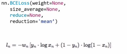
主要参数:

weight:各类别的loss设置权值
ignore_index:忽略某个类别
reduction :计算模式，可为none/sum/ mean
none-逐个元素计算
sum-所有元素求和，返回标量
mean-加权平均，返回标量

测试代码:

# ----------------------------------- 3 BCE Loss -----------------------------------
# flag = 0
flag = 1
if flag:
    inputs = torch.tensor([[1, 2], [2, 2], [3, 4], [4, 5]], dtype=torch.float)
    target = torch.tensor([[1, 0], [1, 0], [0, 1], [0, 1]], dtype=torch.float)

    target_bce = target

    # itarget
    inputs = torch.sigmoid(inputs)

    weights = torch.tensor([1, 1], dtype=torch.float)

    loss_f_none_w = nn.BCELoss(weight=weights, reduction='none')
    loss_f_sum = nn.BCELoss(weight=weights, reduction='sum')
    loss_f_mean = nn.BCELoss(weight=weights, reduction='mean')

    # forward
    loss_none_w = loss_f_none_w(inputs, target_bce)
    loss_sum = loss_f_sum(inputs, target_bce)
    loss_mean = loss_f_mean(inputs, target_bce)

    # view
    print("\nweights: ", weights)
    print("BCE Loss", loss_none_w, loss_sum, loss_mean)

输出：

weights:  tensor([1., 1.])
BCE Loss tensor([[0.3133, 2.1269],
        [0.1269, 2.1269],
        [3.0486, 0.0181],
        [4.0181, 0.0067]]) tensor(11.7856) tensor(1.4732)

手动计算验证：

# --------------------------------- compute by hand
# flag = 0
flag = 1
if flag:

    idx = 0

    x_i = inputs.detach().numpy()[idx, idx]
    y_i = target.numpy()[idx, idx]              #

    # loss
    # l_i = -[ y_i * np.log(x_i) + (1-y_i) * np.log(1-y_i) ]      # np.log(0) = nan
    l_i = -y_i * np.log(x_i) if y_i else -(1-y_i) * np.log(1-x_i)

    # 输出loss
    print("BCE inputs: ", inputs)
    print("第一个loss为: ", l_i)

输出：

weights:  tensor([1., 1.])
BCE Loss tensor([[0.3133, 2.1269],
        [0.1269, 2.1269],
        [3.0486, 0.0181],
        [4.0181, 0.0067]]) tensor(11.7856) tensor(1.4732)
BCE inputs:  tensor([[0.7311, 0.8808],
        [0.8808, 0.8808],
        [0.9526, 0.9820],
        [0.9820, 0.9933]])
第一个loss为:  0.31326166

符号要求。
4.nn. BCEWithLogitsLoss
功能:结合Sigmoid与二分类交叉熵
注意事项:网络最后不加sigmoid函数
在这里插入图片描述
主要参数:

pos_weight :正样本的权值
weight:各类别的loss设置权值
ignore_index: 忽略某个类别
reduction :计算模式，可为none/sum/mean
none-逐个元素计算
sum-所有元素求和，返回标量
mean-加权平均，返回标量

测试代码：

# ----------------------------------- 4 BCE with Logis Loss -----------------------------------
# flag = 0
flag = 1
if flag:
    inputs = torch.tensor([[1, 2], [2, 2], [3, 4], [4, 5]], dtype=torch.float)
    target = torch.tensor([[1, 0], [1, 0], [0, 1], [0, 1]], dtype=torch.float)

    target_bce = target

    # inputs = torch.sigmoid(inputs)

    weights = torch.tensor([1, 1], dtype=torch.float)

    loss_f_none_w = nn.BCEWithLogitsLoss(weight=weights, reduction='none')
    loss_f_sum = nn.BCEWithLogitsLoss(weight=weights, reduction='sum')
    loss_f_mean = nn.BCEWithLogitsLoss(weight=weights, reduction='mean')

    # forward
    loss_none_w = loss_f_none_w(inputs, target_bce)
    loss_sum = loss_f_sum(inputs, target_bce)
    loss_mean = loss_f_mean(inputs, target_bce)

    # view
    print("\nweights: ", weights)
    print(loss_none_w, loss_sum, loss_mean)


# --------------------------------- pos weight

# flag = 0
flag = 1
if flag:
    inputs = torch.tensor([[1, 2], [2, 2], [3, 4], [4, 5]], dtype=torch.float)
    target = torch.tensor([[1, 0], [1, 0], [0, 1], [0, 1]], dtype=torch.float)

    target_bce = target

    # itarget
    # inputs = torch.sigmoid(inputs)

    weights = torch.tensor([1], dtype=torch.float)
    pos_w = torch.tensor([1], dtype=torch.float)        # 3

    loss_f_none_w = nn.BCEWithLogitsLoss(weight=weights, reduction='none', pos_weight=pos_w)
    loss_f_sum = nn.BCEWithLogitsLoss(weight=weights, reduction='sum', pos_weight=pos_w)
    loss_f_mean = nn.BCEWithLogitsLoss(weight=weights, reduction='mean', pos_weight=pos_w)

    # forward
    loss_none_w = loss_f_none_w(inputs, target_bce)
    loss_sum = loss_f_sum(inputs, target_bce)
    loss_mean = loss_f_mean(inputs, target_bce)

    # view
    print("\npos_weights: ", pos_w)
    print(loss_none_w, loss_sum, loss_mean)

输出：


weights:  tensor([1., 1.])
tensor([[0.3133, 2.1269],
        [0.1269, 2.1269],
        [3.0486, 0.0181],
        [4.0181, 0.0067]]) tensor(11.7856) tensor(1.4732)

pos_weights:  tensor([1.])
tensor([[0.3133, 2.1269],
        [0.1269, 2.1269],
        [3.0486, 0.0181],
        [4.0181, 0.0067]]) tensor(11.7856) tensor(1.4732)

这个时候 loss值是一致的，当设置pos_w = torch.tensor([3], dtype=torch.float)时：

weights:  tensor([1., 1.])
tensor([[0.3133, 2.1269],
        [0.1269, 2.1269],
        [3.0486, 0.0181],
        [4.0181, 0.0067]]) tensor(11.7856) tensor(1.4732)

pos_weights:  tensor([3.])
tensor([[0.9398, 2.1269],
        [0.3808, 2.1269],
        [3.0486, 0.0544],
        [4.0181, 0.0201]]) tensor(12.7158) tensor(1.5895)

对应位置上的loss，进行放大了3倍。

四.作业

损失函数的reduction有三种模式，它们的作用分别是什么？
当inputs和target及weight分别如以下参数时，reduction=’mean’模式时，loss是如何计算得到的？
inputs = torch.tensor([[1, 2], [1, 3], [1, 3]], dtype=torch.float)
target = torch.tensor([0, 1, 1], dtype=torch.long)
weights = torch.tensor([1, 2]
测试代码：

import torch
import torch.nn as nn
# fake data
inputs = torch.tensor([[1, 2], [1, 3], [1, 3]], dtype=torch.float)
target = torch.tensor([0, 1, 1], dtype=torch.long)

# ----------------------------------- CrossEntropy loss: reduction -----------------------------------
# def loss function
weights = torch.tensor([1, 2], dtype=torch.float)
loss_f_mean = nn.CrossEntropyLoss(weight=weights, reduction='mean')

# forward
loss_mean = loss_f_mean(inputs, target)

# view
print("\nweights: \n", weights)

# view
# https://pytorch.org/docs/stable/_modules/torch/nn/modules/loss.html#CrossEntropyLoss
# loss(x,class)=weight[class](−x[class]+log(∑ exp(x[j]))) 如果reduction='sum', 那么返回loss(x, class)
# loss_mean = loss(x,class)/ ∑ weight[class]
print("\nCross Entropy Loss:\n ", loss_mean)

输出：


weights: 
 tensor([1., 2.])

Cross Entropy Loss:
  tensor(0.3642)

NotFound1911

关注

0
点赞
踩
3

收藏

觉得还不错? 一键收藏
0
评论
学习笔记|Pytorch使用教程14(损失函数(一))

学习笔记|Pytorch使用教程14本学习笔记主要摘自“深度之眼”，做一个总结，方便查阅。使用Pytorch版本为1.2损失函数概念交叉熵损失函数NLL/BCE/BCEWithLogits Loss一.损失函数概念损失函数:衡量模型输出与真实标签的差异损失函数(Loss Function) :Loss=f(y∧,y)Loss=f\left(y^{\wedge}, y\ri...
复制链接

扫一扫