【机器学习】SoftMax多分类

softMax分类函数

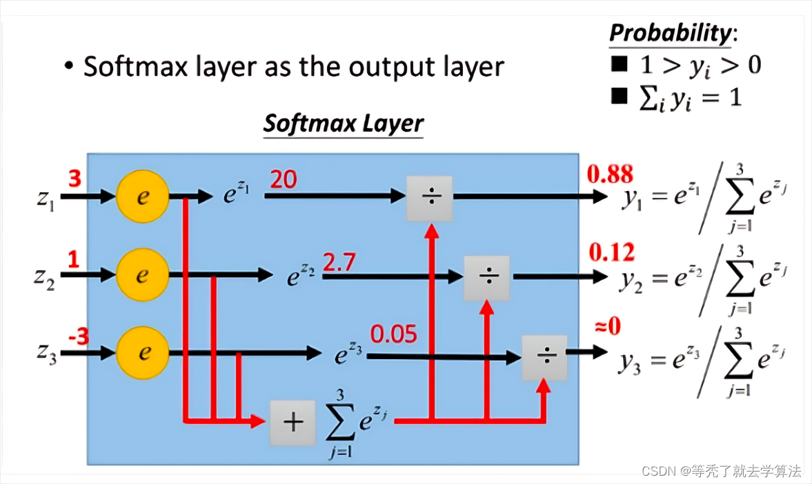
首先给一个图，这个图比较清晰地告诉大家softmax是怎么计算的。

(图片来自网络)

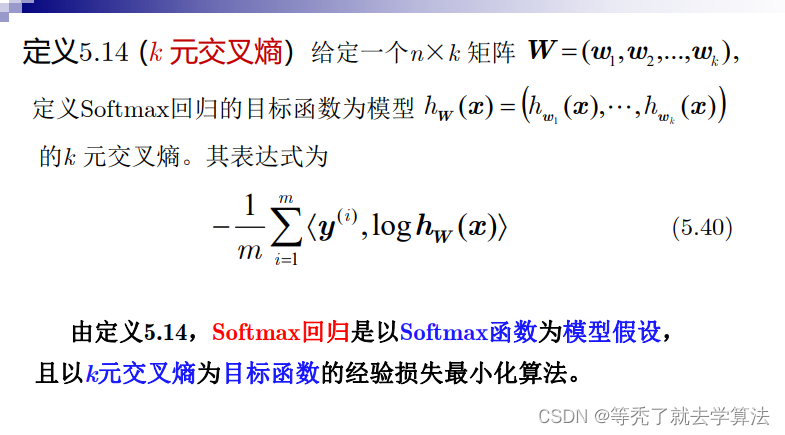
定义：

给定以歌$n\times k$矩阵$W=(w_1,w_2,...,w_k)$,其中，$w_j\in R^n$为$n\times 1$列向量（$1\le j\le k$）,Softmax模型$h_w:R^n\to R^k$为：
$$h_W(x)=(\frac{e^{<w_1,x>}}{{\sum }_{t=1}^k{e}^{<w_t,x>}},\frac{e^{<w_2,x>}}{{\sum }_{t=1}^k{e}^{<w_t,x>}},...,\frac{e^{<w_k,x>}}{{\sum }_{t=1}^k{e}^{<w_t,x>}}{)}_{(样本m\times k)}$$

样本$x_1$的softmax值为：
$$h_W(x_1)=(\frac{e^{<w_1,x_1>}}{{\sum }_{t=1}^k{e}^{<w_t,x_1>}},\frac{e^{<w_2,x_1>}}{{\sum }_{t=1}^k{e}^{<w_t,x_1>}},...,\frac{e^{<w_k,x_1>}}{{\sum }_{t=1}^k{e}^{<w_t,x_1>}}{)}_{(1\times k)}$$
且可知$$\sum _1^k{h}_w(x_1)=1$$

类别数k要小于特征维度n
如果类别数大于特征维度，那么就会出现过多的未知参数需要学习，导致模型过于复杂，难以训练和泛化。因此，通常是将类别数设定为特征维度的一个较小的值，以保证模型的简洁性和可行性。

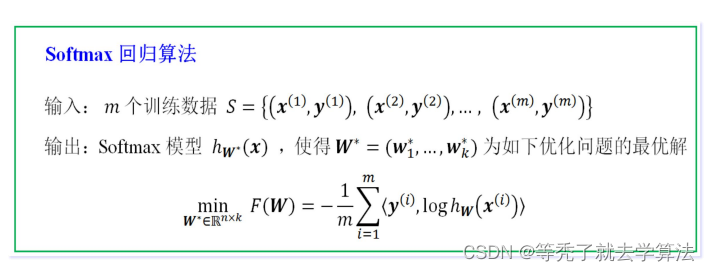
softmax分类损失函数

交叉熵的理论部分在上一篇文章：Logistic回归
前面提到，在多分类问题中，我们经常使用交叉熵作为损失函数
$$Loss=-\sum t_{i}ln{y}_i$$
其中$t_i$表示真实值，$y_i$表示求出的softmax值。当预测第i个时，可以认为$t_i$=1.此时损失函数变成了$$Los{s}_i=-ln{y}_i$$
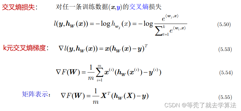
代入$$y_i=h_W(x_i)$$，求梯度
$$▽Los{s}_i=y_i-1$$上面的结果表示，我们只需要正向求出$y_i$，将结果减1就是反向更新的梯度，导数的计算是不是非常简单！

总结一下：

练习题：红酒产地预测

本实验使用softmax回归模型进行红酒品质分类。首先，导入红酒数据，并将类标签转换为one-hot向量表示， 特征组向量前面置1（为了将线性回归b吸收到w中）。

rwine = load_wine()  # 导入红酒数据
X = rwine.data
y = rwine.target
m, n = X.shape
y = convert_to_vectors(y)
X = np.concatenate((np.ones((m, 1)), X), axis=1)

然后，进行数据预处理，包括特征归一化和随机划分训练集和测试集。

# 正则化，原因是e = np.exp(scores)会溢出，将x正则化[]
X = normalize(X)
X_train, X_test, y_train, y_test = train_test_split(X, y, test_size=0.2)

接着，使用softmax回归模型对训练集进行训练，并在测试集上进行预测和模型评估。得到的Accuracy值是：0.9444444444444444

# 使用自定义的SoftMax回归模型
model = SoftmaxRegression()
model.fit(X_train, y_train)
model.predict(X_test)
y_score = model.proba
y_true = max_indices = np.argmax(y_test, axis=1)


# 精确率计算
def t_pre(y_pre, y_true):
    count = 0
    for i in range(len(y_pre)):
        if y_pre[i] - y_true[i] == 0:
            count += 1
    return count


acc = (t_pre(np.argmax(model.proba, axis=1), y_true)) / len(y_true)
print(acc)

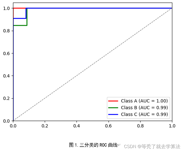
最后，绘制ROC曲线和计算AUC值，以进一步评估模型性能。

# 绘制ROC曲线：调用skelearn库中方法
# 将每个标签作为正例，其他两个标签合并作为负例，计算ROC曲线和AUC值
fpr, tpr, roc_auc = {}, {}, {}
for i in range(3):
    fpr[i], tpr[i], _ = roc_curve(y_true == i, y_score[:, i])
    roc_auc[i] = auc(fpr[i], tpr[i])

plt.figure()
colors = ['red', 'green', 'blue']
labels = ['Class A', 'Class B', 'Class C']
for i in range(3):
    plt.plot(fpr[i], tpr[i], color=colors[i], lw=2,
             label='{0} (AUC = {1:0.2f})'
                   ''.format(labels[i], roc_auc[i]))
plt.plot([0, 1], [0, 1], color='gray', lw=1, linestyle='--')
plt.xlim([0.0, 1.0])
plt.ylim([0.0, 1.05])
plt.legend(loc="lower right")
plt.show()

完整代码：

from sklearn.datasets import load_wine
from sklearn.model_selection import train_test_split
from sklearn.metrics import roc_curve, auc, accuracy_score
import matplotlib.pyplot as plt
import numpy as np




def normalize(X):
    X_min = np.min(X, axis=0)
    X_max = np.max(X, axis=0)
    print(X_max)
    denom = X_max - X_min
    # 将所有分母为零的元素置为一个小值
    denom[denom == 0] = 1e-8
    return (X - X_min) / denom


def softmax(scores):
    e = np.exp(scores)
    s = e.sum(axis=1)
    for i in range(len(s)):
        e[i] /= s[i]
    return e


def threshold(t, proba):
    return (proba >= t).astype(np.int)


def plot_roc_curve(proba, y):
    fpr, tpr = [], []
    for i in range(100):
        z = threshold(0.01 * i, proba)
        tp = (y * z).sum()
        fp = ((1 - y) * z).sum()
        tn = ((1 - y) * (1 - z)).sum()
        fn = (y * (1 - z)).sum()
        fpr.append(1.0 * fp / (fp + tn))
        tpr.append(1.0 * tp / (tp + fn))
    plt.plot(fpr, tpr)
    plt.show()


class SoftmaxRegression:

    def __init__(self):
        self.w = None
        self.proba = None

    def fit(self, X, y, eta_0=50, eta_1=100, N=1000):
        m, n = X.shape
        m, k = y.shape
        w = np.zeros(n * k).reshape(n, k)

        if self.w is None:
            self.w = np.zeros(n * k).reshape(n, k)
        for t in range(N):
            i = np.random.randint(m)
            x = X[i].reshape(1, -1)
            print(x.dot(w))
            proba = softmax(x.dot(w))
            g = x.T.dot(proba - y[i])
            w = w - eta_0 / (t + eta_1) * g
            self.w += w
        self.w /= N

    def predict_proba(self, X):
        return softmax(X.dot(self.w))

    def predict(self, X):
        self.proba = self.predict_proba(X)
        return np.argmax(self.proba, axis=1)


def convert_to_vectors(c):  # 转换成 m*k 矩阵(one-hot向量)， m样本数，k类别数
    # c为类标签列向量 m*1，c[i]{0,1,..,k-1}
    m = len(c)
    k = np.max(c) + 1
    y = np.zeros(m * k).reshape(m, k)
    for i in range(m):
        y[i][c[i]] = 1  # y[i]的第c[i]位置1，其余位为0
    return y


rwine = load_wine()  # 导入红酒数据
X = rwine.data
y = rwine.target
m, n = X.shape
y = convert_to_vectors(y)
X = np.concatenate((np.ones((m, 1)), X), axis=1)
# 正则化，原因是e = np.exp(scores)会溢出，将x正则化[]
X = normalize(X)
X_train, X_test, y_train, y_test = train_test_split(X, y, test_size=0.2)
# 使用自定义的SoftMax回归模型
model = SoftmaxRegression()
model.fit(X_train, y_train)
model.predict(X_test)
y_score = model.proba
y_true = max_indices = np.argmax(y_test, axis=1)


# 精确率计算
def t_pre(y_pre, y_true):
    count = 0
    for i in range(len(y_pre)):
        if y_pre[i] - y_true[i] == 0:
            count += 1
    return count


acc = (t_pre(np.argmax(model.proba, axis=1), y_true)) / len(y_true)
print(acc)

# 绘制ROC曲线：调用skelearn库中方法
# 将每个标签作为正例，其他两个标签合并作为负例，计算ROC曲线和AUC值
fpr, tpr, roc_auc = {}, {}, {}
for i in range(3):
    fpr[i], tpr[i], _ = roc_curve(y_true == i, y_score[:, i])
    roc_auc[i] = auc(fpr[i], tpr[i])

plt.figure()
colors = ['red', 'green', 'blue']
labels = ['Class A', 'Class B', 'Class C']
for i in range(3):
    plt.plot(fpr[i], tpr[i], color=colors[i], lw=2,
             label='{0} (AUC = {1:0.2f})'
                   ''.format(labels[i], roc_auc[i]))
plt.plot([0, 1], [0, 1], color='gray', lw=1, linestyle='--')
plt.xlim([0.0, 1.0])
plt.ylim([0.0, 1.05])
plt.legend(loc="lower right")
plt.show()

1. 在用自定义的Softmax回归，对于没有正则化的X，它在进入softmax（scores）函数，会出现溢出情况，需要控制X.dot(w)的值的大小。这里的正则化是指的数据预处理的归一化（将每个特征值都缩放到0和1之间） 公式：x’ = (x - min(x)) / (max(x) - min(x))，不会影响分类结果（会影响W值，但是并不需要关注W值）
2. ROC曲线：对于多分类的ROC曲线的绘制，可以分别将各个类别作为正例，其他类别作为反例，最后可以取平均AUC值作为该模型的AUC值