ResNet网络详解与keras实现

ResNet网络详解与keras实现

本博客旨在给经典的ResNet网络进行详解与代码实现，如有不足或者其他的见解，请在本博客下面留言。

Resnet网络的概览

1. 为了解决训练很深的网络时候出现的梯度退化(gradient degradation)的问题,Kaiming He提出了Resnet结构。由于使用了残差学习的方法(Resuidal learning)，使得网络的层数得到了大大的提升。
2. ResNet由于使用了shortcut,把原来需要学习逼近的未知函数H(x)恒等映射(Identity mapping),变成了逼近F(x)=H(x)-x的一个函数。作者认为这两种表达的效果相同，但是优化的难度却并不相同，作者假设F(x)的优化会比H(x)简单的多。这一想法也是源于图像处理中的残差向量编码，通过一个reformulation，将一个问题分解成多个尺度直接的残差问题，能够很好的起到优化训练的效果。
3. ResNet针对较深(层数大于等于50)的网络提出了BottleNeck的结构，这个结构可以减少运算的时间复杂度。
4. ResNet里存在两种shortcut,Identity shortcut & Projection shortcut。Identity shortcut使用零填充的方式保证其纬度不变，而Projection shortcut则具有下面的形式$y=F(x,{W_i})+W_sx$来匹配纬度的变换。
5. ResNet这个模型在图像处理的相关任务中具有很好的泛化性，在2015年的ImageNet Recognization,ImageNet detection,ImageNet localization,COCO detection,COCO segmentation等等任务上取得第一的成绩。

在本篇博客中，将对Resnet的结构进行详细的解释，并用代码实现ResNet的网络结构。同时，本文还将引入另一篇论文<>，来更加深入的理解Resnet。本文使用VOC2012的数据集进行网络的训练，验证，与测试。为了快速开发，本次我们把Keras作为代码的框架。

Pascal_VOC数据集

Pascal VOC为图像识别，检测与分割提供了一整套标准化的优秀的数据集，每一年都会举办一次图像识别竞赛。下面是VOC2012，训练集(包括验证集)的下载地址。

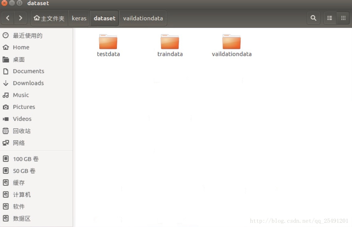
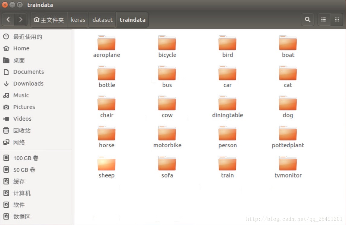
VOC2012里面有20类物体的图片，图片总共有1.7万张。我把数据集分成了3个部分，训练集，验证集，测试集，比例为8:1:1。
下面是部分截图：

第一层目录

---

第二层目录

---

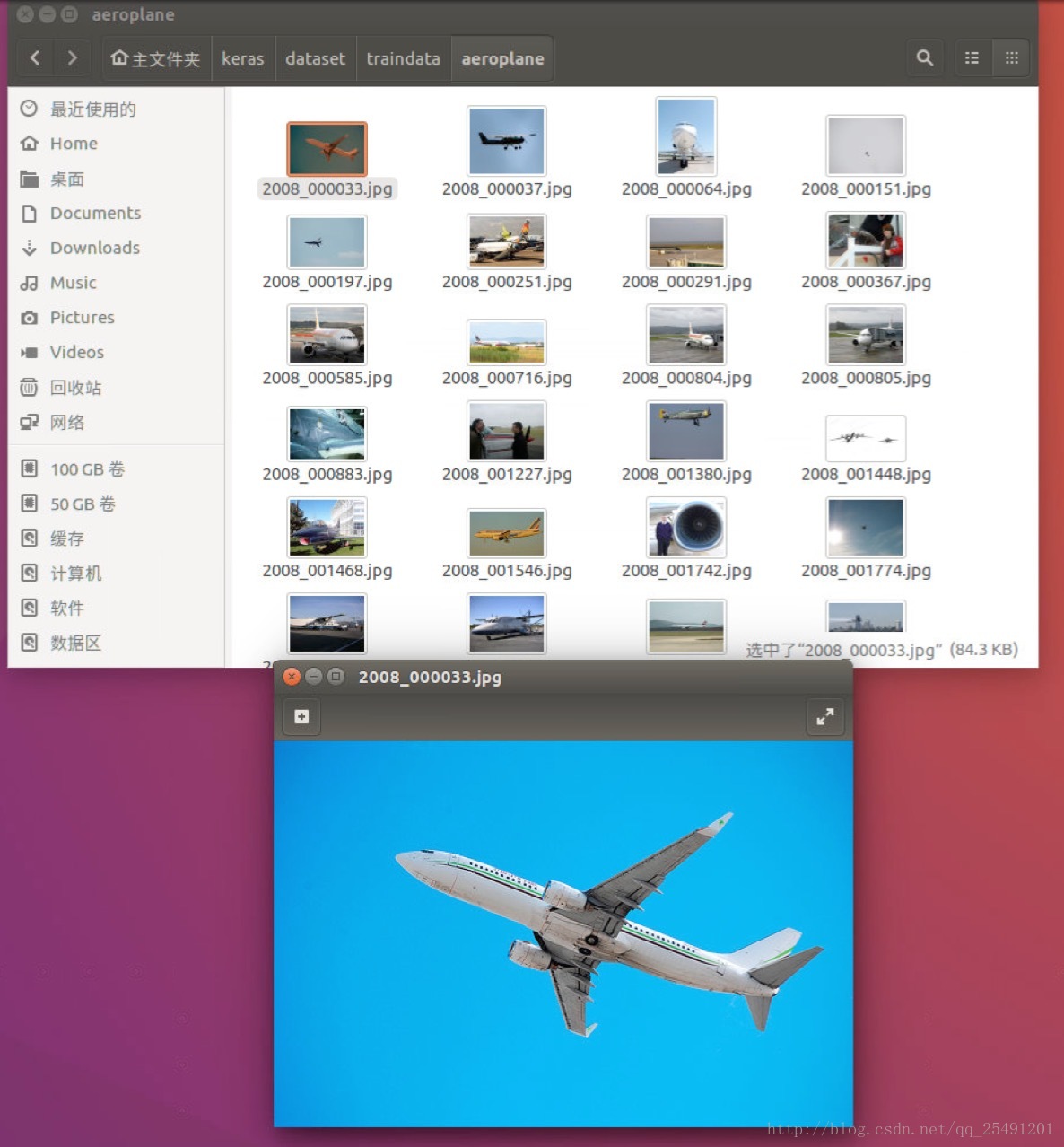
第三层目录

---

接着我们使用keras代码来使用这个数据集，代码如下：

IM_WIDTH=224 #图片宽度
IM_HEIGHT=224 #图片高度
batch_size=32 #批的大小

# train data
train_datagen = ImageDataGenerator(
    width_shift_range=0.1,
    height_shift_range=0.1,
    shear_range=0.1,
    zoom_range=0.1,
    horizontal_flip&