Linear Regression(多变量)

波士顿房产数据(完整数据)

波士顿房价数据集（Boston House Price Dataset）（下载地址：http://t.cn/RfHTAgY）

使用sklearn.datasets.load_boston即可加载相关数据。该数据集是一个回归问题。每个类的观察值数量是均等的，共有 506 个观察，13 个输入变量和1个输出变量。

每条数据包含房屋以及房屋周围的详细信息。其中包含城镇犯罪率，一氧化氮浓度，住宅平均房间数，到中心区域的加权距离以及自住房平均房价等等。

from sklearn.datasets import load_boston
boston = load_boston()
print(boston.data.shape)

(506, 13) #Samples total 506 , Dimensionality 13

from sklearn.datasets import load_boston
import pandas as pd

import matplotlib.pyplot as plt

from sklearn import datasets
from pandas.plotting import scatter_matrix

boston = load_boston()

print('--- %s ---' % 'boston type')
print(type(boston))
print('--- %s ---' % 'boston keys')
print(boston.keys())
print('--- %s ---' % 'boston data')
print(type(boston.data))

print('--- %s ---' % 'boston target')
print(type(boston.target))
print('--- %s ---' % 'boston data shape')
print(boston.data.shape)

print('--- %s ---' % 'boston feature names')
print(boston.feature_names);


X = boston.data
y = boston.target
df = pd.DataFrame(X, columns= boston.feature_names)

print('--- %s ---' % 'df.head')
print(df.head())

— boston type —
<class ‘sklearn.utils.Bunch’>
— boston keys —
dict_keys([‘data’, ‘target’, ‘feature_names’, ‘DESCR’])
— boston data —
<class ‘numpy.ndarray’>
— boston target —
<class ‘numpy.ndarray’>
— boston data shape —
(506, 13)
— boston feature names —
[‘CRIM’ ‘ZN’ ‘INDUS’ ‘CHAS’ ‘NOX’ ‘RM’ ‘AGE’ ‘DIS’ ‘RAD’ ‘TAX’ ‘PTRATIO’
‘B’ ‘LSTAT’]
— df.head —
CRIM ZN INDUS CHAS NOX … RAD TAX PTRATIO B LSTAT
0 0.00632 18.0 2.31 0.0 0.538 … 1.0 296.0 15.3 396.90 4.98
1 0.02731 0.0 7.07 0.0 0.469 … 2.0 242.0 17.8 396.90 9.14
2 0.02729 0.0 7.07 0.0 0.469 … 2.0 242.0 17.8 392.83 4.03
3 0.03237 0.0 2.18 0.0 0.458 … 3.0 222.0 18.7 394.63 2.94
4 0.06905 0.0 2.18 0.0 0.458 … 3.0 222.0 18.7 396.90 5.33

[5 rows x 13 columns]

（参考：https://www.cnblogs.com/wwwjjjnnn/p/7323862.html
https://www.cnblogs.com/python-machine/p/6940578.html
https://www.jianshu.com/p/a9a1ecd7f3eb）

多变量线性回归

多变量线性回归原理回顾

多维特征（Multiple features）

对于一个要度量的对象，一般来说会有不同维度的多个特征。比如之前的房屋价格预测例子中，除了房屋的面积大小，可能还有房屋的年限、房屋的层数等等其他特征：

这里由于特征不再只有一个，引入一些新的记号:

多变量预测函数（Multiple features）

多变量梯度下降（Gradient descent for Multiple variables）

特征缩放（Gradient descent in practice:Feature Scaling）

如果你有一个机器学习问题，这个问题有多个特征，如果你能确保这些特征，都处在一个相近的范围，它的作用是，将多个特征的数据的取值范围处理在相近的范围内，从而使梯度下降更快地收敛。

下图中，左图是以原始数据绘制的代价函数轮廓图，右图为采用特征缩放（都除以最大值）后图像。左图中呈现的图像较扁，相对于使用特征缩放方法的右图，梯度下降算法需要更多次的迭代。

为了优化梯度下降的收敛速度，采用特征缩放的技巧，使各特征值的范围尽量一致。

除了以上图人工选择并除以一个参数的方式，均值归一化(Mean normalization)方法更为便捷，可采用它来对所有特征值统一缩放：

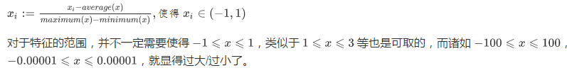
另外注意，一旦采用特征缩放，我们就需对所有的输入采用特征缩放，包括训练集、测试集、预测输入等。

学习速率（Gradient descent in practice:Learning Rate）

我们可以通过绘制代价函数关于迭代次数的图像，可视化梯度下降的执行过程，借助直观的图形来发现代价函数趋向于多少时能趋于收敛，依据图像变化情况，确定诸如学习速率的取值，迭代次数的大小等问题。


对于学习速率 alpha，一般上图展现的为适中情况，下图中，左图可能表明 alpha 过大，代价函数无法收敛，右图可能表明 alpha 过小，代价函数收敛的太慢。当然， alpha足够小时，代价函数在每轮迭代后一定会减少。

特征与多项式回归（Features and polynomial regression）

在特征选取时，我们也可以自己归纳总结，定义一个新的特征，用来取代或拆分旧的一个或多个特征。比如，对于房屋面积特征来说，我们可以将其拆分为长度和宽度两个特征，反之，我们也可以合并长度和宽度这两个特征为面积这一个特征。

线性回归只能以直线来对数据进行拟合，有时候需要使用曲线来对数据进行拟合，即多项式回归(Polynomial Regression)。

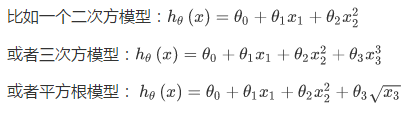
在使用多项式回归时，要记住非常有必要进行特征缩放，比如 的范围为 1-1000，那么 x1^2的范围则为 1- 1000000，不适用特征缩放的话，范围更有不一致，也更易影响效率。

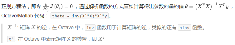
正规方程（Normal Equation）

对于一些线性回归问题来说，正规方程法给出了一个更好的解决问题的方式。

下表列出了正规方程法与梯度下降算法的对比

(参考：1.https://mp.weixin.qq.com/s?__biz=MzU4NzE2MTgyNQ%3D%3D&chksm=fdf10b62ca868274719eeac0508ae4779e7378d78969a5ebf2fd539ab724a0491028735c2316&idx=1&mid=2247484140&sn=659fcd22edb5be0448cc756d6507dcfb
2.https://scruel.gitee.io/ml-andrewng-notes/week2.html#header-n2
3.https://www.jianshu.com/p/ebc333be0462
4.https://blog.csdn.net/louishao/article/details/54670081
5https://www.cnblogs.com/jianxinzhou/p/4055333.html
6.https://blog.csdn.net/qq_33297776/article/details/52243144
7.https://www.jianshu.com/p/2bd439f0a5c4
8http://cw.hubwiz.com/card/c/56d644b4ecba4b4d31cd280a/1/5/2/)

多变量线性回归代码实现

import numpy as np
from sklearn import datasets

dataset = datasets.load_boston()
print(dataset.get('feature_names'))
# 使用第6-8列feature，即AGE(1940年以前建成的自住单位的比例),
# DIS(距离五个波士顿就业中心的加权距离),RAD(距离高速公路的便利指数)
X = dataset.data[:, 5:8]
# 为X增加一列全为1，来求偏置项
X = np.column_stack((X, np.ones(len(X))))
y = dataset.target

# 划分训练集和测试集
X_train = X[:-20]
X_test = X[-20:]
y_train = y[:-20]
y_test = y[-20:]

X_train = np.mat(X_train)
y_train = np.mat(y_train).T

xTx = X_train.T * X_train
w = 0
if np.linalg.det(xTx) == 0.0:
    print('xTx不可逆')
else:
    w = np.ravel(xTx.I * (X_train.T * y_train))
coef_ = w[:-1]
intercept_ = w[-1]

# 去掉添加的那一列1
X_train = X_train[:, 0:3]
X_test = X_test[:, 0:3]

y_test_pred = coef_[0] * X_test[:, 0] + coef_[1] * X_test[:, 1] + coef_[2] * X_test[:, 2] + intercept_

# 矩阵转回数组
X_train = np.ravel(X_train).reshape(-1, 3)
y_train = np.ravel(y_train)

print('Coefficients: ', coef_)
print('Intercept:', intercept_)
print('the model is: y = ', coef_, '* X + ', intercept_)
# 均方误差
print("Mean squared error: %.2f" % np.average((y_test - y_test_pred) ** 2))

Coefficients: [ 8.46020754 -0.09742681 -0.48029222]
Intercept: -22.0839441928
the model is: y = [ 8.46020754 -0.09742681 -0.48029222] * X + -22.0839441928
Mean squared error: 10.33

参考：https://github.com/Sun-Shuai/machine-learning/tree/master/linear regression

与 from sklearn.linear_model import LinearRegression的对比:

from sklearn import datasets, linear_model
from sklearn.metrics import mean_squared_error, r2_score
import warnings

# 不想看到warning，添加以下代码忽略它们
warnings.filterwarnings(action="ignore", module="sklearn")

dataset = datasets.load_boston()
print(dataset.get('feature_names'))
# 使用第6-8列feature，即AGE(1940年以前建成的自住单位的比例),
# DIS(距离五个波士顿就业中心的加权距离),RAD(距离高速公路的便利指数)
X = dataset.data[:, 5:8]
y = dataset.target

# 划分训练集和测试集
X_train = X[:-20]
X_test = X[-20:]
y_train = y[:-20]
y_test = y[-20:]

regr = linear_model.LinearRegression()
regr.fit(X_train, y_train)
y_test_pred = regr.predict(X_test)

print('Coefficients: ', regr.coef_)
print('Intercept:', regr.intercept_)
print('the model is: y = ', regr.coef_, '* X + ', regr.intercept_)
# 均方误差
print("Mean squared error: %.2f" % mean_squared_error(y_test, y_test_pred))
# r2 score，0,1之间，越接近1说明模型越好，越接近0说明模型越差
print('Variance score: %.2f' % r2_score(y_test, y_test_pred))

[‘CRIM’ ‘ZN’ ‘INDUS’ ‘CHAS’ ‘NOX’ ‘RM’ ‘AGE’ ‘DIS’ ‘RAD’ ‘TAX’ ‘PTRATIO’
‘B’ ‘LSTAT’]
Coefficients: [ 8.46020754 -0.09742681 -0.48029222]
Intercept: -22.0839441928
the model is: y = [ 8.46020754 -0.09742681 -0.48029222] * X + -22.0839441928
Mean squared error: 10.33
Variance score: 0.56

数据标准化

from sklearn import datasets;
from sklearn.svm import SVR;
from sklearn.cross_validation import train_test_split;
from sklearn.preprocessing import StandardScaler;    #用于数据预处理的数据放缩函数
from numpy import *;

house_dataset = datasets.load_boston()
house_data = house_dataset.data;
house_price = house_dataset.target;
x_train,x_test,y_train,y_test=train_test_split(house_data,house_price,test_size=0.2);
#StandardScaler是数据放缩的其中一种方案，即f(x)=(x-平均值)/标准差
scaler = StandardScaler();
#在数据模型建立时，只能使用训练组数据，因此使用训练组数据的标准差进行标准化
scaler.fit(x_train);
#对训练组和测试组的输入数据进行标准化，即f(训练组或测试组数据)=(训练组或测试组数据-训练组或测试组平均值)/训练组标准差
x_train = scaler.transform(x_train);
x_test = scaler.transform(x_test);

网格搜索调参

有关模型的参数调优过程，即网格搜索/交叉验证
最简单的网格搜索：两层for循环

# naive grid search implementation
from sklearn.datasets import load_iris
from sklearn.svm import SVC
from sklearn.model_selection import train_test_split
iris = load_iris()
X_train, X_test, y_train, y_test = train_test_split(iris.data, iris.target, random_state=0)
print("Size of training set: %d   size of test set: %d" % (X_train.shape[0], X_test.shape[0]))

best_score = 0
for gamma in [0.001, 0.01, 0.1, 1, 10, 100]:
    for C in [0.001, 0.01, 0.1, 1, 10, 100]:
        # for each combination of parameters
        # train an SVC
        svm = SVC(gamma=gamma, C=C)
        svm.fit(X_train, y_train)
        # evaluate the SVC on the test set 
        score = svm.score(X_test, y_test)
        # if we got a better score, store the score and parameters
        if score > best_score:
            best_score = score
            best_parameters = {'C': C, 'gamma': gamma}

print("best score: ", best_score)
print("best parameters: ", best_parameters)

#Output:
#Size of training set: 112   size of test set: 38
#best score:  0.973684210526
#best parameters:  {'gamma': 0.001, 'C': 100}

网格搜索内部嵌套了交叉验证：

mport numpy as np
from sklearn.datasets import load_iris
from sklearn.svm import SVC
from sklearn.model_selection import cross_val_score
iris = load_iris()
X_trainval, X_test, y_trainval, y_test = train_test_split(iris.data, iris.target, random_state=0)   #总集——>训练验证集+测试集
X_train, X_valid, y_train, y_valid = train_test_split(X_trainval, y_trainval, random_state=1)   #训练验证集——>训练集+验证集
best_score = 0
for gamma in [0.001, 0.01, 0.1, 1, 10, 100]:
    for C in [0.001, 0.01, 0.1, 1, 10, 100]:
        svm = SVC(gamma=gamma, C=C)
        scores = cross_val_score(svm, X_trainval, y_trainval, cv=5)   #在训练集和验证集上进行交叉验证
        score = np.mean(scores)   # compute mean cross-validation accuracy
        if score > best_score:   
            best_score = score
            best_parameters = {'C': C, 'gamma': gamma}

构造参数字典,代替双层for循环进行网格搜索：

param_grid = {'C': [0.001, 0.01, 0.1, 1, 10, 100],'gamma': [0.001, 0.01, 0.1, 1, 10, 100]}
from sklearn.model_selection import GridSearchCV
from sklearn.svm import SVC
X_trainvalid, X_test, y_trainvalid, y_test = train_test_split(iris.data, iris.target, random_state=0)   #default=0.25
grid_search = GridSearchCV(SVC(), param_grid, cv=5)   #网格搜索+交叉验证
grid_search.fit(X_trainvalid, y_trainvalid)

嵌套交叉验证：字典参数+cross_val_score：

from sklearn.datasets import load_iris
from sklearn.model_selection import GridSearchCV
from sklearn.model_selection import cross_val_score
from sklearn.svm import SVC
param_grid = {'C': [0.001, 0.01, 0.1, 1, 10, 100],'gamma': [0.001, 0.01, 0.1, 1, 10, 100]}
scores = cross_val_score(GridSearchCV(SVC(), param_grid, cv=5), iris.data, iris.target, cv=5)   
#选定网格搜索的每一组超参数,对训练集与测试集的交叉验证(cross_val_score没指定数据集合分割的默认情况)
print("Cross-validation scores: ", scores)
print("Mean cross-validation score: ", scores.mean())

reference:https://blog.csdn.net/weixin_41829272/article/details/81330207
GridSearchCV :https://blog.csdn.net/sunshunli/article/details/81814574
实战演练网格搜索与模型调参:https://www.jianshu.com/p/98a7caffd12b
调参必备–Grid Search网格搜索 https://www.jianshu.com/p/55b9f2ea283b
【scikit-learn】网格搜索来进行高效的参数调优 https://blog.csdn.net/jasonding1354/article/details/50562522