Gaussian Process(高斯过程) GPSS暑校笔记总计Ⅰ（英文版）——高斯过程介绍

What is Machine Learning?

$$\text{data}+\text{model}\Rightarrow \text{prediction}$$

• $\text{data}$ : observations, could be actively or passively
  acquired (meta-data).
• $\text{model}$ : assumptions, based on previous experience (other data!
  transfer learning etc), or beliefs about the regularities of
  the universe. Inductive bias.
• $\text{prediction}$ : an action to be taken or a categorization or a
  quality score.

Two important Gaussian Properties

• Sum of Gaussianv

  Sum of Gaussian variables is also Gaussian.

$$y_i\sim \mathcal{N}({\mu }_i,{\sigma }_i^2)$$

And the sum is distributed as

$$\sum y_i\sim \mathcal{N}(\sum {\mu }_i,\sum {\sigma }_i^2)$$

Aside: As sum increase, sum of non-Gaussian, finite variance variables is also Gaussian because of central limit theorem.

• Scaling a Gaussian
  Scaling a Gaussian leads to a Gaussian.

  $$\omega \ast y\sim \mathcal{N}(\omega \mu ,{\omega }^2{\sigma }^2)$$

The central limit theorem (CLT) establishes that, in some situations, when independent random variables are added, their properly normalized sum tends toward a normal distribution (informally a “bell curve”) even if the original variables themselves are not normally distributed.

Prior Distribution

• Bayesian inference requires a prior on the parameters.
• The prior represents your belief before you see the data of the
  likely value of the parameters.
• For linear regression, consider a Gaussian prior on the intercept:

$$c\sim \mathcal{N}(0,{\alpha }_1)$$

Posterior Distribution

• Posterior distribution is found by combining the prior with
  the likelihood.
• Posterior distribution is your belief after you see the data of
  the likely value of the parameters.
• The posterior is found through Bayes’ Rule
  $$p(c|y)=\frac{p(y|c)p(c)}{p(y)}$$
  The $p(y|c)$ likelihood is not a density over $c$, it’s a function of $c$. Here, $c$ is a parameter of this density. The normalization step, e.g. find the suitable way to compute the $p(y)$ is the most difficult setp.

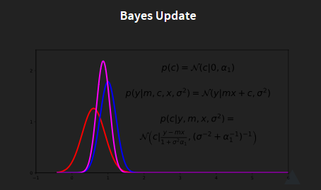
The red line describe the probablity for $c$ with:
$$p(c)=\mathcal{N}(c|0,{\alpha }_1)$$
the blue line stands for the observation, with:
$$p(y|m,c,x,{\sigma }^2)=\mathcal{N}(y|mx+c,{\sigma }^2)$$
Note that, this is a likelihood function over $c$ not a distribution.
based on the bayes’rule, the posterior could be written as:
$$P(c|y,m,x,{\sigma }^2)=\mathcal{N}(c|\frac{y-mx}{1+{\sigma }^2}\alpha ,({\sigma }^{-2}+{\alpha }_1^{-1}{)}^{-1})$$
Math Trick:
$$p(c)=\frac{1}{\sqrt{2\pi {\alpha }_1}}\exp \left(-\frac{1}{2{\alpha }_1}{c}^2\right)$$
$$p(\mathbf{y}|\mathbf{x},c,m,{\sigma }^2)=\frac{1}{{\left(2\pi {\sigma }^2\right)}^{\frac{n}{2}}}\exp \left(-\frac{1}{2{\sigma }^2}\sum _{i=1}^n(y_i-m{x}_i-c{)}^2\right)$$
$$p(c|\mathbf{y},\mathbf{x},m,{\sigma }^2)=\frac{p(\mathbf{y}|\mathbf{x},c,m,{\sigma }^2)p(c)}{p(\mathbf{y}|\mathbf{x},m,{\sigma }^2)}$$

$$p(c|\mathbf{y},\mathbf{x},m,{\sigma }^2)=\frac{p(\mathbf{y}|\mathbf{x},c,m,{\sigma }^2)p(c)}{\int p(\mathbf{y}|\mathbf{x},c,m,{\sigma }^2)p(c)\text{d}c}$$
$$p(c|\mathbf{y},\mathbf{x},m,{\sigma }^2)\propto p(\mathbf{y}|\mathbf{x},c,m,{\sigma }^2)p(c)$$

$$\begin{array}{rl}\log p(c|\mathbf{y},\mathbf{x},m,{\sigma }^2)=& -\frac{1}{2{\sigma }^2}\sum _{i=1}^n(y_i-c-m{x}_i{)}^2-\frac{1}{2{\alpha }_1}{c}^2+\text{const}\\ =& -\frac{1}{2{\sigma }^2}\sum _{i=1}^n(y_i-m{x}_i{)}^2-\left(\frac{n}{2{\sigma }^2}+\frac{1}{2{\alpha }_1}\right)c^2\\ & +c\frac{{\sum }_{i=1}^n(y_i-m{x}_i)}{{\sigma }^2},\end{array}$$

complete the square of the quadratic form to obtain
$$\log p(c|\mathbf{y},\mathbf{x},m,{\sigma }^2)=-\frac{1}{2{\tau }^2}(c-\mu {)}^2+\text{const}$$
where
$${\tau }^2={\left(n{\sigma }^{-2}+{\alpha }_1^{-1}\right)}^{-1}$$
and

$\mu =\frac{{\tau }^2}{{\sigma }^2}{\sum }_{i=1}^n(y_i-m{x}_i)$.

Piror comes from the model, where we think about it. And likelihood is coming from the data.

Stages to Derivation of the Posterior

• Multiply likelihood by prior
  • they are “exponentiated quadratics”, the answer is always also an exponentiated quadratic because
    $$\exp (a^2)\exp (b^2)=\exp (a^2+b^2)$$
• Complete the square to get the resulting density in the form of a Gaussian.
• Recognise the mean and (co)variance of the Gaussian. This is the estimate of the posterior.

Multivariate Regression Likelihood

• Noise corrupted data point
  $$y_i=w^T{X}_{i,:}+{ϵ}_i$$
• Multivariate regression likelihood:
  $$p(y|X,w)=\frac{1}{(2\pi {\sigma }^2)}exp(-\frac{1}{2{\sigma }^2}\sum (y_i-w^T{x}_{i,:}{)}^2)$$
• Multivariate Gaussian piroi:
  $$p(w)=\frac{1}{(2\pi {\sigma }^2{)}^{p/2}}exp(-\frac{1}{2{\sigma }^2}{w}^{T}w)$$

The independent multivariate Gaussian could be seen as the independent Gaussian and multiple them and rotate the results.

Independent Gaussians:

$$p(w,h)=\frac{1}{\sqrt{2\pi {\alpha }_1}\sqrt{2\pi {\alpha }_2}}\exp (-\frac{1}{2}(\frac{(w-{\mu }_1{)}^2}{{\sigma }_1^2}+\frac{(h-{\mu }_2{)}^2}{{\sigma }_2^2}))$$

and we can write it with linear algebra form:
$$p(w,h)=\frac{1}{\sqrt{2\pi {\alpha }_1}\sqrt{2\pi {\alpha }_2}}\exp (-\frac{1}{2}(\left[\begin{array}{c}w\\ h\end{array}\right]-\left[\begin{array}{c}{u}_1\\ u_2\end{array}\right]{)}^T(\left[\begin{array}{cc}{\sigma }_1& 0\\ 0& {\sigma }_2\end{array}\right]\left[\begin{array}{c}w\\ h\end{array}\right]-\left[\begin{array}{c}{u}_1\\ u_2\end{array}\right]))$$

and then, rename it:
$$p(y)=\frac{1}{|2\pi \ast D{|}^{\frac{1}{2}}}\exp (-\frac{1}{2}(y-\mu {)}^T{D}^{-1}(Y-\mu ))$$
$|D|$ means the determinant of the matrix.

Correlated Gaussian

Form correlated from original by rotating the data space using matrx R.
$$p(y)=\frac{1}{|2\pi \ast D{|}^{\frac{1}{2}}}\exp (-\frac{1}{2}(R^{T}y-R^T\mu {)}^T{D}^{-1}(R^{T}Y-R^T\mu ))$$
$$p(y)=\frac{1}{|2\pi \ast D{|}^{\frac{1}{2}}}\exp (-\frac{1}{2}(y-\mu {)}^{T}R{D}^{-1}{R}^T(Y-\mu ))$$
this gives a covariance matric:
$$C^{-1}=R{D}^{-1}{R}^T$$
which in some view is the result of the principal compoment.

Multivariate Consequence

if
$$x\sim \mathcal{N}(\mu ,\Sigma )$$
and
$$y=Wx$$
then
$$y\sim \mathcal{N}(W\mu ,W\Sigma W^T)$$

we can say the first equaption is the prior of $x$, the second is the likelihood, the last is the marginal of $y$. If we set $\mu =0,\Sigma =I$, so it is just the inverse of PCA.

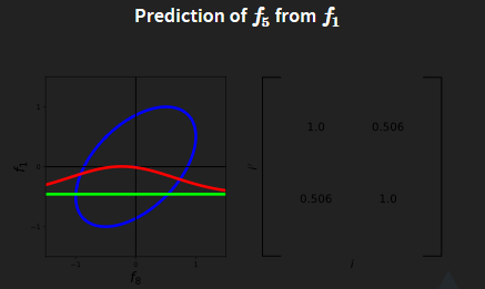
Prediction with Correlated Gaussians

• Prediction of ${\mathbf{f}}_{\ast }$ from $\mathbf{f}$ requires multivariate conditional density.

• Multivariate conditional density is also Gaussian.
  $$p({\mathbf{f}}_{\ast }|\mathbf{f})=\mathcal{N}\left({\mathbf{f}}_{\ast }|{\mathbf{K}}_{\ast ,\mathbf{f}}{\mathbf{K}}_{\mathbf{f},\mathbf{f}}^{-1}\mathbf{f},{\mathbf{K}}_{\ast ,\ast }-{\mathbf{K}}_{\ast ,\mathbf{f}}{\mathbf{K}}_{\mathbf{f},\mathbf{f}}^{-1}{\mathbf{K}}_{\mathbf{f},\ast }\right)$$

• Here covariance of joint density is given by
  $$\mathbf{K}=\left[\begin{array}{cc}{\mathbf{K}}_{\mathbf{f},\mathbf{f}}& {\mathbf{K}}_{\ast ,\mathbf{f}}\\ {\mathbf{K}}_{\mathbf{f},\ast }& {\mathbf{K}}_{\ast ,\ast }\end{array}\right]$$

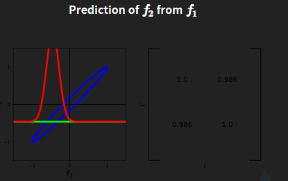
Take the picture as the example:

since that example is in 1D, all the values are scalar. $f=f1=-0.4$, $K_{f,f}=1,K_{\ast ,f}=0.98,K_{\ast ,\ast }=1$, so
$$p(p_2|p_1)=\mathcal{N}(p_2|0.98\ast 1\ast (-0.4),1-0.98\ast 1\ast 0.98)$$
$$p(p_2|p_1)=\mathcal{N}(p_2|-0.392,0.0396)$$
the variance is 0.0396, and the standard variance is 0.2.