（七）PCA数据降维

一、PCA（Principle Component Analysis）

1.1 PCA的作用

作用：主成分分析；数据降维，便于理解，减少计算用时

基本原理：数据所有样本点映射到一个新轴，保持所有样本间方差最大，此时样本保持原有特性最多，区分度也最大，实现了降维

1.2 主成分：特征各自的方差百分比（贡献率），越大权重越大

from  sklearn.decomposition  import  PCA
import  numpy as np

# 生成一个10行4维的随机矩阵
x = np.random.rand(10,4)
x
'''
array([[0.49616494, 0.09861945, 0.04795112, 0.73494469],
       [0.73209859, 0.24548772, 0.32351747, 0.20813443],
       [0.44778574, 0.86454078, 0.124517  , 0.2339795 ],
       [0.06958403, 0.65457276, 0.52441239, 0.88351689],
       [0.03411929, 0.48477378, 0.15958519, 0.839266  ],
       [0.96134173, 0.60006946, 0.76167245, 0.6257422 ],
       [0.16255676, 0.64281049, 0.83714188, 0.50882656],
       [0.58254891, 0.17365182, 0.94439864, 0.13799818],
       [0.28306401, 0.55308271, 0.80268313, 0.68167844],
       [0.30686136, 0.91480948, 0.42434956, 0.02401578]])
'''

# 不传参数表示对所有特征进行主成分分析
pca  = PCA()
pca.fit(x)
'''
PCA(copy=True, iterated_power='auto', n_components=None, random_state=None,
    svd_solver='auto', tol=0.0, whiten=False)
'''

# 返回模型的各个特征向量
pca.components_
'''
array([[-0.61502763,  0.12109321, -0.47645582,  0.61649599],
       [ 0.41634831, -0.45285324, -0.7820247 , -0.10007697],
       [-0.1763014 ,  0.65985771, -0.39755788, -0.61274248],
       [ 0.64599762,  0.58723775, -0.0580944 ,  0.48421477]])
'''

# 返回每个主成分各自的方差百分比（贡献率），从大到小
# 如果选前三个主成分，则这3维数据约占原始数据0.373+0.271+0.256=90%的信息
pca.explained_variance_ratio_
'''
array([0.37256121, 0.27136823, 0.25580559, 0.10026497])
'''

# sum(pca.explained_variance_ratio_)
# 1.0000000000000002

二、手写数字识别 

2.1 准备

import numpy as np
import matplotlib.pyplot as plt
from sklearn import datasets

digits = datasets.load_digits()
x = digits.data
y = digits.target

from sklearn.model_selection import train_test_split

x_train, x_test, y_train, y_test = train_test_split(x, y, test_size=0.2, random_state=666)
x_train.shape
'''
(1437, 64)    #总计1437个手写数据图片，每个图片大小8x8
'''

2.2 数据可视化

import  matplotlib.pyplot  as plt

fig, ax = plt.subplots(nrows=6,ncols=6,sharex='all',sharey='all')
ax = ax.flatten()
for i in range(36):
    img = x_train[i].reshape(8, 8)
    ax[i].imshow(img,cmap='Greys')
    ax[0].set_xticks([])
    ax[0].set_yticks([])
    
plt.tight_layout()
plt.show()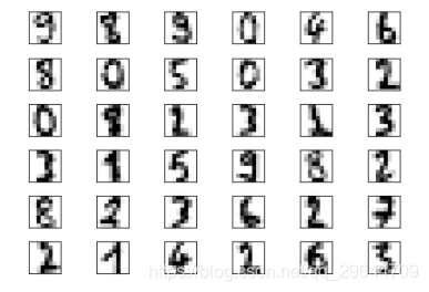

2.3 使用PCA降维，用KNeighborsClassifier预测

    结论：n_components 取值不同对执行影响不同

• n_components 越大保留的原样本信息越多，预测结果越准确，但用时越多
• n_components 越小，丢失的原样本信息越多，预测结果越低，用时减少

from sklearn.decomposition import PCA

 n_components = 2 、 4、 8、 12、 16、 22时预测值变大

pca = PCA(n_components=2)
pca.fit(x_train)
x_train_reduction = pca.transform(x_train)
x_test_reduction = pca.transform(x_test)

knn_clf = KNeighborsClassifier()
knn_clf.fit(x_train_reduction, y_train)
knn_clf.score(x_test_reduction, y_test)
'''
n_components = 2    预测值：0.6055555555555555
n_components = 4    预测值：0.875
n_components = 8    预测值：0.9472222222222222
n_components = 12   预测值：0.9722222222222222
n_components = 16   预测值：0.9833333333333333
n_components = 22   预测值：0.9861111111111112
'''

2.4  n_components取值：整数或者浮点型

# 如果把64个特征全部信息使用，找到每一个主成分对方差的解释程度
# 数据由大到小排列
pca = PCA(n_components=64)
pca.fit(x_train)
pca.explained_variance_ratio_
'''
array([1.45064600e-01, 1.37142456e-01, 1.19680004e-01, 8.43768923e-02,
       5.87005941e-02, 5.01797333e-02, 4.34065700e-02, 3.61375740e-02,
       3.39661991e-02, 3.00599249e-02, 2.38906921e-02, 2.29417581e-02,
       1.81335935e-02, 1.78403959e-02, 1.47411385e-02, 1.41290045e-02,
       1.29333094e-02, 1.25283166e-02, 1.01123057e-02, 9.08986879e-03,
       8.98365069e-03, 7.72299807e-03, 7.62541166e-03, 7.09954951e-03,
       6.96433125e-03, 5.84665284e-03, 5.77225779e-03, 5.07732970e-03,
       4.84364707e-03...])
'''

np.sum(pca.explained_variance_ratio_)   # 1.0

# n_components 取值逐渐变大时，取得的主成分对原数据方差的解释比例增大
# n_components 越大，数据越完整，越小数据丢失信息可能越多
plt.figure(figsize=(10,6))
plt.rcParams['font.sans-serif']=['SimHei']
plt.xlabel("主成分个数")
plt.ylabel("解释方差比例")
plt.plot([i for i in range(x_train.shape[1])],
        [np.sum(pca.explained_variance_ratio_[:i+1]) for i in range(x_train.shape[1])])
plt.show()

# n_components 赋 整数 k 时,提取前k个特征（主成分）
# n_components 赋 0-1之间的 浮点数如0.95，被选择的所有主成分包含原变量所有信息的95%
pca = PCA(n_components=0.95)
pca.fit(x_train)
pca.explained_variance_ratio_

# 28个主成分保留了原数据0.95的信息，只丢失了5%原数据信息
pca.n_components_
'''
28   # 当n_components=0.95时，对应选取了28个主成分，从64维降到了28维
'''

三、mnist数据集

mnist数据集：由60000个训练样本和10000个测试样本组成；

每个图像的高度为28像素，宽度为28像素，总计784像素。每个像素都有一个与之关联的像素值，表示该像素的亮度或暗度，数字越高表示像素越暗。此像素值是0到255之间的整数（含0和255）；

训练集中的每个像素列都有一个类似pixelx的名称，其中x是0到783之间的整数（含0和783）。为了在图像上定位该像素，假设我们将x分解为x = i * 28 + j，其中i和j是0到27之间（包括0和27）的整数。然后，pixelx位于28 x 28矩阵的第i行和第j列（索引为零）上。

import  numpy  as  np
from sklearn.datasets import fetch_openml
mnist = fetch_openml("mnist_784")

mnist.keys()
'''
dict_keys(['data', 'target', 'frame', 'feature_names', 'target_names', 'DESCR', 'details', 'categories', 'url'])
'''

x = mnist['data']
y = mnist['target']
print(x.shape)
print(y.shape)
'''
(70000, 784)
(70000,)
'''

x_train = np.array(x[:60000], dtype=float)
y_train = np.array(y[:60000], dtype=float)
x_test = np.array(x[60000:], dtype=float)
y_test = np.array(y[60000:], dtype=float)

3.1 图形化前24个样例

import  matplotlib.pyplot  as plt
#可视化样本 前24个
fig, ax = plt.subplots(nrows=4,ncols=6,sharex='all',sharey='all')
ax = ax.flatten()
for i in range(24):
    img = x_train[i].reshape(28, 28)
    ax[i].imshow(img,cmap='Greys')
    
plt.tight_layout()
plt.show()

 

3.2 未进行PCA降维：训练和验证花费了大量时间

from sklearn.neighbors import KNeighborsClassifier

knn_clf = KNeighborsClassifier()
%time knn_clf.fit(x_train, y_train)
'''
Wall time: 1min 2s
KNeighborsClassifier(algorithm='auto', leaf_size=30, metric='minkowski',
                     metric_params=None, n_jobs=None, n_neighbors=5, p=2,
                     weights='uniform')
'''

%time knn_clf.score(x_test, y_test)
'''
Wall time: 13min 57s
0.9688
'''

3.3 使用PCA降维：精度容忍范围内，用时大大减小

# ------PCA降维
from sklearn.decomposition import PCA

# 保留原数据 90% 的特性，从784维降到87维
pca = PCA(0.9)
pca.fit(x_train)
x_train_reduction = pca.transform(x_train)
x_train_reduction.shape
'''
(60000, 87)
'''

# ------训练
from sklearn.neighbors import KNeighborsClassifier

knn_clf = KNeighborsClassifier()
%time knn_clf.fit(x_train_reduction, y_train)
'''
Wall time: 2.65 s
KNeighborsClassifier(algorithm='auto', leaf_size=30, metric='minkowski',
                     metric_params=None, n_jobs=None, n_neighbors=5, p=2,
                     weights='uniform')
'''

# ------测试
x_test_reduction= pca.transform(x_test)

%time knn_clf.score(x_test_reduction, y_test)
'''
Wall time: 1min 28s
0.9728
'''