误差反向传播之BP算法和梯度下降

我们使用损失函数作为模型的评价准则，衡量一个模型的工作能力。这样问题就变成了一个数学问题，类似于二阶导数求最值点。我们使用优化器（optim）对优化目标（loss function）进行优化，损失函数f(x)取值越小，模型性能越好。

梯度下降：梯度是一个向量，表示某一函数在该点处的方向导数沿着该方向取得最大值，即函数在该点处沿着该方向（此梯度的方向）变化最快，变化率最大（为该梯度的模）。那么我们不停的沿着梯度的反方向前进，函数取值就会不断下降。

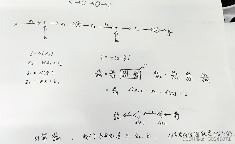
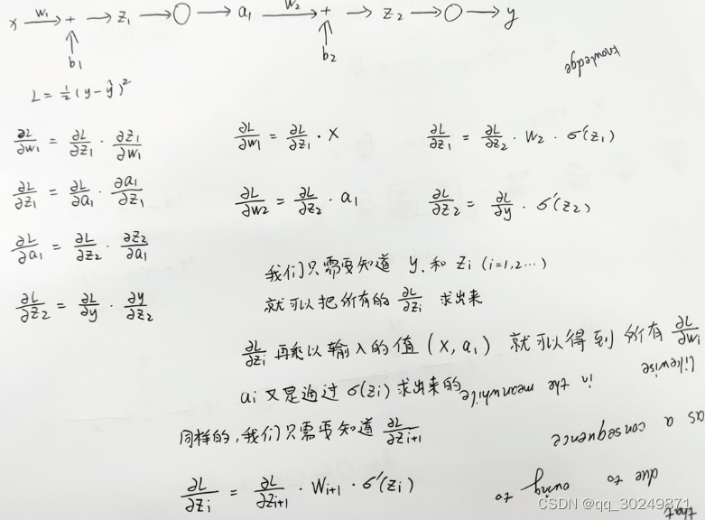
BP算法：利用链式法则，反向传播，求出模型任一变量（w，b）针对损失函数的梯度。

所有变量都沿着梯度的反方向前进，函数取值一定会下降。

代码实现
信号前向传播时需要记录a和z，方便误差反向传播使用。

def backprop(self, x, y):
        """Return a tuple ``(nabla_b, nabla_w)`` representing the
        gradient for the cost function C_x.  ``nabla_b`` and
        ``nabla_w`` are layer-by-layer lists of numpy arrays, similar
        to ``self.biases`` and ``self.weights``."""
        nabla_b = [np.zeros(b.shape) for b in self.biases]
        nabla_w = [np.zeros(w.shape) for w in self.weights]
        # feedforward
        activation = x
        activations = [x] # list to store all the activations, layer by layer
        zs = [] # list to store all the z vectors, layer by layer
        for b, w in zip(self.biases, self.weights):
            z = np.dot(w, activation)+b
            zs.append(z)
            activation = sigmoid(z)
            activations.append(activation)
        # backward pass
        delta = self.cost_derivative(activations[-1], y) * \
            sigmoid_prime(zs[-1])
        nabla_b[-1] = delta
        nabla_w[-1] = np.dot(delta, activations[-2].transpose())
        # Note that the variable l in the loop below is used a little
        # differently to the notation in Chapter 2 of the book.  Here,
        # l = 1 means the last layer of neurons, l = 2 is the
        # second-last layer, and so on.  It's a renumbering of the
        # scheme in the book, used here to take advantage of the fact
        # that Python can use negative indices in lists.
        for l in xrange(2, self.num_layers):
            z = zs[-l]
            sp = sigmoid_prime(z)
            delta = np.dot(self.weights[-l+1].transpose(), delta) * sp
            nabla_b[-l] = delta
            nabla_w[-l] = np.dot(delta, activations[-l-1].transpose())
        return (nabla_b, nabla_w)