从几何角度重新看线性分类器

最近在一本机器学习的书籍上偶然看到了一个很有新颖的想法，绝对让你眼前一亮。从几何角度重新构造一个基本的线性分类器，一般有关机器学习的书籍所讲到的线性分类器都是形如 y=w.*x+t,w代表权重系数，t是分类阈值，一般通过最小化损失函数(误差平方和)，然后通过梯度下降法求得参数w和阈值t。

另一种思路是从几何角度来看待这个问题。线性分类器一般是在实例空间中画一个分类超平面，w从几何角度来看是超平面的法向量，w与超平面垂直。实际上w是有正例的质心向量p减去反例的质心向量n，根据向量的减法，本质上w的方向就是从n指向p，这样w的方向就确定了，确定一个超平面还需要阈值t的值，如果自己画图的话，可以看到1/2*(p+n)恰好在超平面上，这样阈值t = w.*x = (p-n).*1/2(p + n),在判别测试集上实例的类别时候，只需要判断w.*x>t是否成立（也即(p-n).x>t）,若成立则为正例，否则为反例。

专门比较了Logistic分类器和这个方法的分类性能，发现性能大致相同，在以下截图中可以看到。这个思想很精巧！！！

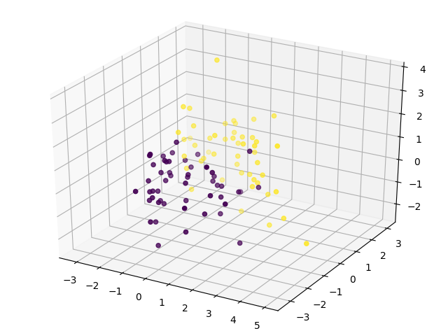
构造的二类数据（3个特征）分布如下图所示:

测试的性能如下图所示:

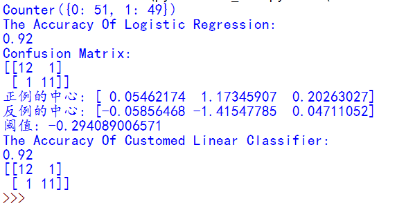
可以看到二者准确率都是92%。难道你不点个赞惊叹一下吗？？？？

# !/usr/bin/env python
# -*- coding:utf-8 -*- 
# Author: wsw
# 自定义线性分类器
from sklearn.datasets import make_classification
from sklearn.metrics import confusion_matrix, classification_report, accuracy_score
from sklearn.linear_model import LogisticRegression
from sklearn.model_selection import train_test_split
import numpy as np
from collections import Counter
import matplotlib.pyplot as plt
# 导入3D画图模块
from mpl_toolkits.mplot3d import Axes3D
# 构造一个二类数据集
rowdata, label = make_classification(100, n_features=3, n_informative=2, n_redundant=0, random_state=33)
c = Counter(label)
print(c)
fig = plt.figure()
ax = Axes3D(fig)
# 将数据点在三维空间显示分布
ax.scatter(rowdata[:, 0], rowdata[:, 1], rowdata[:, 2], c=label)

xtrain, xtest, ytrain, ytest = train_test_split(rowdata, label, test_size=0.25, random_state=22)
# 调用Logsitic分类器
lr = LogisticRegression()
lr.fit(xtrain, ytrain)
lr_predict = lr.predict(xtest)
print('The Accuracy Of Logistic Regression:')
print(lr.score(xtest, ytest))
print('Confusion Matrix:')
print(confusion_matrix(ytest, lr_predict, labels=[0, 1]))

# 自定义线性分类器
# 找到正例的索引
index1 = np.where(label == 1)
# 找到反例的索引
index2 = np.where(label == 0)
# 得到正例的质心
pos_medoid = np.mean(rowdata[index1[0], :], axis=0)
# 得到反例的质心
neg_medoid = np.mean(rowdata[index2[0], :], axis=0)
print('正例的中心:', pos_medoid)
print('反例的中心:', neg_medoid)

# 思想w.*x=t,t是分类阈值，w即分类器的系数权重，与分类超平面垂直(即法平面)
# w = p - n(向量相减，指向正例p)
# 1/2(p+n)恰好在直线上，所以可以确定阈值t=(p-n).*1/2(p+n)
w = pos_medoid - neg_medoid
t = np.dot(w, 1/2*(pos_medoid+neg_medoid))
print('阈值:', t)

# 测试性能
customed_predict = []
for point in xtest:
	if np.dot(w, point) > t:
		customed_predict.append(1)
	else:
		customed_predict.append(0)

# 得到性能
print('The Accuracy Of Customed Linear Classifier:')
print(accuracy_score(ytest, customed_predict))
print(confusion_matrix(ytest, customed_predict))
plt.show()